Setup environment
# Load packages
library(tidyverse)  # importing, transforming, and visualizing data frames
## ── Attaching packages ─────────────────────────────────────── tidyverse 1.3.0 ──## ✓ ggplot2 3.3.3 ✓ purrr 0.3.4
## ✓ tibble 3.0.6 ✓ dplyr 1.0.4
## ✓ tidyr 1.1.2 ✓ stringr 1.4.0
## ✓ readr 1.4.0 ✓ forcats 0.5.1## ── Conflicts ────────────────────────────────────────── tidyverse_conflicts() ──
## x dplyr::filter() masks stats::filter()
## x dplyr::lag() masks stats::lag()library(here) # (relative) file paths## here() starts at /Users/leonreteig/AB-tDCSlibrary(knitr) # R notebook output
library(scales) # Percentage axis labels ##
## Attaching package: 'scales'## The following object is masked from 'package:purrr':
##
## discard## The following object is masked from 'package:readr':
##
## col_factorlibrary(broom) # transform model outputs into data frames
library(ggm) # partial correlations
library(BayesFactor) # Bayesian statistics## Loading required package: coda## Loading required package: Matrix##
## Attaching package: 'Matrix'## The following objects are masked from 'package:tidyr':
##
## expand, pack, unpack## ************
## Welcome to BayesFactor 0.9.12-4.2. If you have questions, please contact Richard Morey (richarddmorey@gmail.com).
##
## Type BFManual() to open the manual.
## ************library(metafor) # meta-analysis## Loading 'metafor' package (version 2.4-0). For an overview
## and introduction to the package please type: help(metafor).library(predictionInterval) # prediction intervals (for correlations)
library(TOSTER) # equivalence tests
library(pwr) # power analysis
library(knitrhooks) # printing in rmarkdown outputs
output_max_height()
# Source functions
source(here("src", "func", "behavioral_analysis.R")) # loading data and calculating measures
knitr::read_chunk(here("src", "func", "behavioral_analysis.R")) # display code from file in this notebook
load_data_path <- here("src","func","load_data.Rmd") # for rerunning and displaying
source(here("src", "lib", "appendixCodeFunctionsJeffreys.R")) # replication Bayes factors## Loading required package: hypergeoprint(sessionInfo())## R version 3.6.2 (2019-12-12) ## Platform: x86_64-apple-darwin15.6.0 (64-bit) ## Running under: macOS 10.16 ## ## Matrix products: default ## BLAS: /Library/Frameworks/R.framework/Versions/3.6/Resources/lib/libRblas.0.dylib ## LAPACK: /Library/Frameworks/R.framework/Versions/3.6/Resources/lib/libRlapack.dylib ## ## locale: ## [1] en_US.UTF-8/en_US.UTF-8/en_US.UTF-8/C/en_US.UTF-8/en_US.UTF-8 ## ## attached base packages: ## [1] stats graphics grDevices datasets utils methods base ## ## other attached packages: ## [1] hypergeo_1.2-13 knitrhooks_0.0.4 pwr_1.3-0 ## [4] TOSTER_0.3.4 predictionInterval_1.0.0 metafor_2.4-0 ## [7] BayesFactor_0.9.12-4.2 Matrix_1.3-2 coda_0.19-4 ## [10] ggm_2.5 broom_0.7.4.9000 scales_1.1.1 ## [13] knitr_1.31 here_1.0.1 forcats_0.5.1 ## [16] stringr_1.4.0 dplyr_1.0.4 purrr_0.3.4 ## [19] readr_1.4.0 tidyr_1.1.2 tibble_3.0.6 ## [22] ggplot2_3.3.3 tidyverse_1.3.0 ## ## loaded via a namespace (and not attached): ## [1] httr_1.4.2 jsonlite_1.7.2 elliptic_1.4-0 modelr_0.1.8 ## [5] gtools_3.8.2 assertthat_0.2.1 renv_0.12.5-72 cellranger_1.1.0 ## [9] yaml_2.2.1 pillar_1.4.7 backports_1.2.1 lattice_0.20-41 ## [13] glue_1.4.2 digest_0.6.27 rvest_0.3.6 colorspace_2.0-0 ## [17] htmltools_0.5.1.1 pkgconfig_2.0.3 haven_2.3.1 bookdown_0.21 ## [21] mvtnorm_1.1-1 MatrixModels_0.5-0 generics_0.1.0 ellipsis_0.3.1 ## [25] withr_2.4.1 pbapply_1.4-3 cli_2.3.0 magrittr_2.0.1 ## [29] crayon_1.4.1 readxl_1.3.1 evaluate_0.14 fs_1.5.0 ## [33] nlme_3.1-152 MASS_7.3-53.1 xml2_1.3.2 MBESS_4.8.0 ## [37] tools_3.6.2 hms_1.0.0 lifecycle_1.0.0 munsell_0.5.0 ## [41] reprex_1.0.0 compiler_3.6.2 jquerylib_0.1.4 contfrac_1.1-12 ## [45] rlang_0.4.10 grid_3.6.2 rstudioapi_0.13 igraph_1.2.6 ## [49] rmarkdown_2.11 gtable_0.3.0 deSolve_1.28 DBI_1.1.1 ## [53] R6_2.5.0 lubridate_1.7.9.2 rprojroot_2.0.2 stringi_1.5.3 ## [57] parallel_3.6.2 rmdformats_1.0.2 Rcpp_1.0.6 vctrs_0.3.6 ## [61] dbplyr_2.1.0 tidyselect_1.1.0 xfun_0.21
Load task data
Study 2
The following participants are excluded from further analysis at this point, because of incomplete data:
S03,S14,S29,S38,S43,S46: their T1 performance in session 1 was less than 63% correct, so they were not invited back. This cutoff was determined based on a separate pilot study with 10 participants. It is two standard deviations below the mean of that sample.S25has no data for session 2, as they stopped responding to requests for scheduling the sessionS31was excluded as a precaution after session 1, as they developed a severe headache and we could not rule out the possibility this was related to the tDCS
dataDir_study2 <- here("data") # root folder with AB task data
subs_incomplete <- c("S03", "S14", "S25", "S29", "S31", "S38", "S43", "S46") # don't try to load data from these participants
df_study2 <- load_data_study2(dataDir_study2, subs_incomplete) %>%
  filter(complete.cases(.)) %>% # discard rows with data from incomplete subjects
   # recode first.session ("anodal" or "cathodal") to session.order ("anodal first", "cathodal first")
  mutate(first.session = parse_factor(paste(first.session, "first"),
                                      levels = c("anodal first", "cathodal first"))) %>%
  rename(session.order = first.session)
n_study2 <- n_distinct(df_study2$subject) # number of subjects in study 2kable(head(df_study2,13), digits = 1, caption = "Data frame for study 2")| subject | session.order | stimulation | block | lag | trials | T1 | T2 | T2.given.T1 |
|---|---|---|---|---|---|---|---|---|
| S01 | anodal first | anodal | pre | 3 | 118 | 0.8 | 0.4 | 0.4 |
| S01 | anodal first | anodal | pre | 8 | 60 | 0.8 | 0.8 | 0.8 |
| S01 | anodal first | anodal | tDCS | 3 | 126 | 0.8 | 0.3 | 0.3 |
| S01 | anodal first | anodal | tDCS | 8 | 65 | 0.8 | 0.7 | 0.7 |
| S01 | anodal first | anodal | post | 3 | 122 | 0.8 | 0.2 | 0.3 |
| S01 | anodal first | anodal | post | 8 | 61 | 0.7 | 0.7 | 0.7 |
| S01 | anodal first | cathodal | pre | 3 | 116 | 0.8 | 0.4 | 0.4 |
| S01 | anodal first | cathodal | pre | 8 | 60 | 0.7 | 0.8 | 0.8 |
| S01 | anodal first | cathodal | tDCS | 3 | 129 | 0.7 | 0.4 | 0.4 |
| S01 | anodal first | cathodal | tDCS | 8 | 64 | 0.7 | 0.8 | 0.9 |
| S01 | anodal first | cathodal | post | 3 | 128 | 0.6 | 0.4 | 0.4 |
| S01 | anodal first | cathodal | post | 8 | 62 | 0.7 | 0.8 | 0.8 |
| S02 | cathodal first | anodal | pre | 3 | 124 | 1.0 | 0.8 | 0.8 |
The data has the following columns:
- subject: Participant ID, e.g.
S01,S12 - session.order: Whether participant received
anodalorcathodaltDCS in the first session (anodal_firstvs.cathodal_first). - stimulation: Whether participant received
anodalorcathodaltDCS - block: Whether data is before (
pre), during (tDCS) or after (post`) tDCS - lag: Whether T2 followed T1 after two distractors (lag
3) or after 7 distractors (lag8) - trials: Number of trials per lag that the participant completed in this block
- T1: Proportion of trials (out of
trials) in which T1 was identified correctly - T2: Proportion of trials (out of
trials) in which T2 was identified correctly - T2.given.T1: Proportion of trials which T2 was identified correctly, out of the trials in which T1 was idenitified correctly (T2|T1).
The number of trials vary from person-to-person, as some completed more trials in a 20-minute block than others (because responses were self-paced):
df_study2 %>%
  group_by(lag) %>%
  summarise_at(vars(trials), funs(mean, min, max, sd)) %>%
  kable(caption = "Descriptive statistics for trial counts per lag", digits = 0)
## Warning: `funs()` was deprecated in dplyr 0.8.0.
## Please use a list of either functions or lambdas:
##
## # Simple named list:
## list(mean = mean, median = median)
##
## # Auto named with `tibble::lst()`:
## tibble::lst(mean, median)
##
## # Using lambdas
## list(~ mean(., trim = .2), ~ median(., na.rm = TRUE))| lag | mean | min | max | sd |
|---|---|---|---|---|
| 3 | 130 | 78 | 163 | 17 |
| 8 | 65 | 39 | 87 | 9 |
Study 1
These data were used for statistical analysis in London & Slagter (2021)1, and were processed by the lead author:
dataPath_study1 <- here("data","AB-tDCS_study1.txt")
data_study1_fromDisk <- read.table(dataPath_study1, header = TRUE, dec = ",")
glimpse(data_study1_fromDisk)
## Rows: 34 ## Columns: 120 ## $ SD_T10.3313, 0.0289, -0.8027, -0.5381, -2.… ## $ MeanBLT1Acc 0.8800, 0.8600, 0.8050, 0.8225, 0.665… ## $ First_Session 1, 2, 1, 1, 2, 1, 2, 1, 2, 2, 1, 2, 1… ## $ fileno pp4, pp6, pp7, pp9, pp10, pp11, pp12,… ## $ AB_HighLow 2, 1, 2, 1, 1, 1, 1, 1, 2, 1, 1, 2, 1… ## $ vb_T1_2_NP 0.925, 0.875, 0.825, 0.625, 0.650, 0.… ## $ vb_T1_4_NP 0.800, 0.825, 0.825, 0.825, 0.675, 0.… ## $ vb_T1_10_NP 0.925, 0.925, 0.800, 0.775, 0.825, 0.… ## $ vb_T1_4_P 0.850, 0.900, 0.825, 0.775, 0.625, 0.… ## $ vb_T1_10_P 0.825, 0.900, 0.775, 0.825, 0.625, 0.… ## $ vb_NB_2_NP 0.1351, 0.3429, 0.3636, 0.3600, 0.346… ## $ vb_NB_4_NP 0.3125, 0.5455, 0.5455, 0.3030, 0.296… ## $ vb_NB_10_NP 0.8378, 0.8108, 0.9688, 0.6129, 0.727… ## $ vb_NB_4_P 0.2941, 0.5278, 0.6061, 0.3226, 0.520… ## $ vb_NB_10_P 0.8485, 0.7778, 0.9032, 0.8182, 0.680… ## $ VB_AB 0.7027, 0.4680, 0.6051, 0.2529, 0.381… ## $ VB_REC 0.5253, 0.2654, 0.4233, 0.3099, 0.431… ## $ VB_PE -0.0184, -0.0177, 0.0606, 0.0196, 0.2… ## $ tb_T1_2_NP 0.775, 0.875, 0.675, 0.725, 0.475, 0.… ## $ tb_T1_4_NP 0.825, 0.825, 0.700, 0.750, 0.675, 0.… ## $ tb_T1_10_NP 0.875, 0.900, 0.700, 0.825, 0.500, 0.… ## $ tb_T1_4_P 0.875, 0.800, 0.700, 0.775, 0.650, 0.… ## $ tb_T1_10_P 0.850, 0.925, 0.800, 0.825, 0.625, 0.… ## $ tb_NB_2_NP 0.1290, 0.5143, 0.2222, 0.0690, 0.315… ## $ tb_NB_4_NP 0.3333, 0.5455, 0.6071, 0.1333, 0.370… ## $ tb_NB_10_NP 0.8286, 0.8611, 0.8571, 0.5152, 0.850… ## $ tb_NB_4_P 0.3143, 0.6250, 0.5357, 0.4839, 0.538… ## $ tb_NB_10_P 0.8529, 0.7568, 0.9375, 0.6667, 0.680… ## $ TB_AB 0.6995, 0.3468, 0.6349, 0.4462, 0.534… ## $ TB_REC 0.4952, 0.3157, 0.2500, 0.3818, 0.479… ## $ TB_PE -0.0190, 0.0795, -0.0714, 0.3505, 0.1… ## $ nb_T1_2_NP 0.850, 0.850, 0.650, 0.725, 0.675, 0.… ## $ nb_T1_4_NP 0.800, 0.850, 0.725, 0.675, 0.575, 0.… ## $ nb_T1_10_NP 0.925, 0.825, 0.750, 0.850, 0.725, 0.… ## $ nb_T1_4_P 0.850, 0.900, 0.675, 0.750, 0.875, 0.… ## $ nb_T1_10_P 0.900, 0.825, 0.750, 0.800, 0.550, 0.… ## $ nb_NB_2_NP 0.0588, 0.4412, 0.4615, 0.1034, 0.296… ## $ nb_NB_4_NP 0.0938, 0.4412, 0.2414, 0.1481, 0.478… ## $ nb_NB_10_NP 0.8649, 0.7576, 0.9667, 0.6765, 0.896… ## $ nb_NB_4_P 0.4118, 0.7222, 0.4815, 0.3667, 0.685… ## $ nb_NB_10_P 0.8333, 0.8485, 0.8333, 0.7188, 0.818… ## $ NB_AB 0.8060, 0.3164, 0.5051, 0.5730, 0.600… ## $ NB_REC 0.7711, 0.3164, 0.7253, 0.5283, 0.418… ## $ NB_PE 0.3180, 0.2810, 0.2401, 0.2185, 0.207… ## $ vd_T1_2_NP 0.925, 0.875, 0.800, 0.850, 0.575, 0.… ## $ vd_T1_4_NP 0.850, 0.825, 0.825, 0.925, 0.700, 0.… ## $ vd_T1_10_NP 0.850, 0.900, 0.825, 0.925, 0.750, 0.… ## $ vd_T1_4_P 0.925, 0.775, 0.825, 0.750, 0.650, 0.… ## $ vd_T1_10_P 0.925, 0.800, 0.725, 0.950, 0.575, 0.… ## $ vd_NB_2_NP 0.0541, 0.2857, 0.3125, 0.1765, 0.173… ## $ vd_NB_4_NP 0.2941, 0.4848, 0.4545, 0.2432, 0.428… ## $ vd_NB_10_NP 1.0000, 0.6667, 0.9394, 0.7838, 0.766… ## $ vd_NB_4_P 0.5135, 0.6774, 0.4848, 0.5000, 0.500… ## $ vd_NB_10_P 0.8919, 0.8125, 0.9310, 0.8421, 0.608… ## $ VD_AB 0.9459, 0.3810, 0.6269, 0.6073, 0.592… ## $ VD_REC 0.7059, 0.1818, 0.4848, 0.5405, 0.338… ## $ VD_PE 0.2194, 0.1926, 0.0303, 0.2568, 0.071… ## $ td_T1_2_NP 0.950, 0.775, 0.625, 0.775, 0.525, 0.… ## $ td_T1_4_NP 0.975, 0.800, 0.800, 0.750, 0.625, 0.… ## $ td_T1_10_NP 0.975, 0.900, 0.800, 0.850, 0.575, 0.… ## $ td_T1_4_P 0.875, 0.800, 0.800, 0.800, 0.600, 0.… ## $ td_T1_10_P 0.875, 0.800, 0.850, 0.700, 0.525, 0.… ## $ td_NB_2_NP 0.1579, 0.3226, 0.5200, 0.1290, 0.142… ## $ td_NB_4_NP 0.4615, 0.4375, 0.3750, 0.2333, 0.320… ## $ td_NB_10_NP 0.9487, 0.6944, 0.9375, 0.6471, 0.826… ## $ td_NB_4_P 0.4571, 0.3750, 0.5625, 0.4063, 0.583… ## $ td_NB_10_P 0.8857, 0.6875, 0.8529, 0.7143, 0.666… ## $ TD_AB 0.7908, 0.3719, 0.4175, 0.5180, 0.683… ## $ TD_REC 0.4872, 0.2569, 0.5625, 0.4137, 0.506… ## $ TD_PE -0.0044, -0.0625, 0.1875, 0.1729, 0.2… ## $ nd_T1_2_NP 0.700, 0.800, 0.650, 0.775, 0.425, 0.… ## $ nd_T1_4_NP 0.850, 0.850, 0.725, 0.850, 0.650, 0.… ## $ nd_T1_10_NP 0.800, 0.825, 0.800, 0.850, 0.600, 0.… ## $ nd_T1_4_P 0.850, 0.800, 0.775, 0.775, 0.725, 0.… ## $ nd_T1_10_P 0.850, 0.750, 0.800, 0.850, 0.675, 0.… ## $ nd_NB_2_NP 0.0000, 0.2188, 0.2692, 0.0968, 0.235… ## $ nd_NB_4_NP 0.3824, 0.5000, 0.5172, 0.2353, 0.384… ## $ nd_NB_10_NP 0.8750, 0.5758, 0.8125, 0.7941, 0.708… ## $ nd_NB_4_P 0.4118, 0.5000, 0.5806, 0.5484, 0.482… ## $ nd_NB_10_P 0.9118, 0.7667, 0.8438, 0.8235, 0.629… ## $ ND_AB 0.8750, 0.3570, 0.5433, 0.6973, 0.473… ## $ ND_REC 0.4926, 0.0758, 0.2953, 0.5588, 0.323… ## $ ND_PE 0.0294, 0.0000, 0.0634, 0.3131, 0.098… ## $ AnoMinBl_Lag2_NP -0.01, 0.17, -0.14, -0.29, -0.03, 0.0… ## $ AnoMinBl_Lag10_NP -0.01, 0.05, -0.11, -0.10, 0.12, -0.0… ## $ CathoMinBl_Lag2_NP 0.10, 0.04, 0.21, -0.05, -0.03, 0.09,… ## $ CathoMinBl_Lag10_NP -0.05, 0.03, 0.00, -0.14, 0.06, 0.00,… ## $ Tijdens_AnoMinBl_Lag2_NP -0.01, 0.17, -0.14, -0.29, -0.03, 0.0… ## $ Tijdens_AnoMinBl_Lag10_NP -0.01, 0.05, -0.11, -0.10, 0.12, -0.0… ## $ Tijdens_CathoMinBl_Lag2_NP 0.10, 0.04, 0.21, -0.05, -0.03, 0.09,… ## $ Tijdens_CathoMinBl_Lag10_NP -0.05, 0.03, 0.00, -0.14, 0.06, 0.00,… ## $ Tijdens_AnoMinBL_AB 0.00, -0.12, 0.03, 0.19, 0.15, -0.08,… ## $ Tijdens_CathoMinBL_AB -0.16, -0.01, -0.21, -0.09, 0.09, -0.… ## $ Na_AnoMinBL_AB 0.10, -0.15, -0.10, 0.32, 0.22, -0.04… ## $ Na_CathoMinBL_AB -0.07, -0.02, -0.08, 0.09, -0.12, -0.… ## $ Tijdens_AnoMinBL_PE 0.00, 0.10, -0.13, 0.33, -0.06, -0.06… ## $ Tijdens_CathoMinBL_PE -0.22, -0.26, 0.16, -0.08, 0.19, -0.0… ## $ Na_CathoMinBL_PE -0.19, -0.19, 0.03, 0.06, 0.03, 0.31,… ## $ Na_AnoMinBL_PE 0.34, 0.30, 0.18, 0.20, -0.02, 0.06, … ## $ Tijdens_AnoMinBL_REC -0.03, 0.05, -0.17, 0.07, 0.05, 0.07,… ## $ Tijdens_CathoMinBL_REC -0.22, 0.08, 0.08, -0.13, 0.17, -0.03… ## $ Na_CathoMinBL_REC -0.21, -0.11, -0.19, 0.02, -0.01, 0.1… ## $ Na_AnoMinBL_REC 0.25, 0.05, 0.30, 0.22, -0.01, 0.13, … ## $ T1_Lag2_Tijdens_Ano_Min_BL_NP -0.15, 0.00, -0.15, 0.10, -0.18, 0.00… ## $ T1_Lag2_Tijdens_Catho_Min_BL_NP 0.02, -0.10, -0.18, -0.08, -0.05, -0.… ## $ T1_Lag2_Na_Ano_Min_BL_NP -0.08, -0.03, -0.18, 0.10, 0.03, -0.1… ## $ T1_Lag2_Na_Catho_Min_BL_NP -0.23, -0.08, -0.15, -0.08, -0.15, -0… ## $ T1_Lag4_Tijdens_Ano_Min_BL_NP 0.02, 0.00, -0.13, -0.08, 0.00, 0.05,… ## $ T1_Lag4_Tijdens_Catho_Min_BL_NP 0.13, -0.02, -0.02, -0.18, -0.08, 0.0… ## $ T1_Lag4_Na_Catho_Min_BL_NP 0.00, 0.03, -0.10, -0.08, -0.05, 0.13… ## $ T1_Lag4_Na_Ano_Min_BL_NP 0.00, 0.03, -0.10, -0.15, -0.10, 0.02… ## $ Mean_BL_PE 0.10, 0.09, 0.05, 0.14, 0.15, -0.13, … ## $ ZVB_AB 0.72613, -0.71847, 0.12559, -2.04185,… ## $ ZTB_AB 0.97738, -1.74477, 0.47867, -0.97793,… ## $ ZNB_AB 1.24043, -1.72891, -0.58440, -0.17267… ## $ ZVD_AB 2.47191, -1.64491, 0.14714, 0.00446, … ## $ ZTD_AB 1.39518, -1.23661, -0.94993, -0.31845… ## $ ZND_AB 2.00765, -1.59142, -0.29725, 0.77327,… ## $ VB_T1_Acc_ 0.87, 0.89, 0.81, 0.77, 0.68, 0.95, 0… ## $ VD_T1_Acc_ 0.90, 0.84, 0.80, 0.88, 0.65, 0.90, 0…
We’ll use only a subset of columns, with the header structure block/stim_target_lag_prime, where:
- block/stim is either:
vb: “anodal” tDCS, “pre” block (before tDCS)tb: “anodal” tDCS, “tDCS” block (during tDCS)nb: “anodal” tDCS, “post” block (after tDCS)vd: “cathodal” tDCS, “pre” block (before tDCS)td: “cathodal” tDCS, “tDCS” block (during tDCS)nd: “cathodal” tDCS, “post” block (after tDCS)
- target is either:
T1(T1 accuracy): proportion of trials in which T1 was identified correctlyNB(T2|T1 accuracy): proportion of trials in which T2 was identified correctly, given T1 was identified correctly
- lag is either:
2(lag 2), when T2 followed T1 after 1 distractor4(lag 4), when T2 followed T1 after 3 distractors10, (lag 10), when T2 followed T1 after 9 distractors
- prime is either:
P(prime): when the stimulus at lag 2 (in lag 4 or lag 10 trials) had the same identity as T2NP(no prime) when this was not the case. Study 2 had no primes, so we’ll only keep these.
We’ll also keep two more columns: fileno (participant ID) and First_Session (1 meaning participants received anodal tDCS in the first session, 2 meaning participants received cathodal tDCS in the first session).
Reformat
Now we’ll reformat the data to match the data frame for study 2:
format_study2 <- function(df) {
  df %>%
    select(fileno, First_Session, ends_with("_NP"), -contains("Min")) %>% # keep only relevant columns
    gather(key, accuracy, -fileno, -First_Session) %>% # make long form
    # split key column to create separate columns for each factor
    separate(key, c("block", "stimulation", "target", "lag"), c(1,3,5)) %>% # split after 1st, 3rd, and 5th character
    # convert to factors, relabel levels to match those in study 2
    mutate(block = factor(block, levels = c("v", "t", "n"), labels = c("pre", "tDCS", "post")),
           stimulation = factor(stimulation, levels = c("b_", "d_"), labels = c("anodal", "cathodal")),
           lag = factor(lag, levels = c("_2_NP", "_4_NP", "_10_NP"), labels = c(2, 4, 10)),
           First_Session = factor(First_Session, labels = c("anodal first","cathodal first"))) %>%
    spread(target, accuracy) %>% # create separate columns for T2.given.T1 and T1 performance
    rename(T2.given.T1 = NB, session.order = First_Session, subject = fileno)# rename columns to match those in study 2
}
df_study1 <- format_study2(data_study1_fromDisk)
n_study1 <- n_distinct(df_study1$subject) # number of subjects in study 1kable(head(df_study1,19), digits = 1, caption = "Data frame for study 1")| subject | session.order | block | stimulation | lag | T2.given.T1 | T1 |
|---|---|---|---|---|---|---|
| pp10 | cathodal first | pre | anodal | 2 | 0.3 | 0.6 |
| pp10 | cathodal first | pre | anodal | 4 | 0.3 | 0.7 |
| pp10 | cathodal first | pre | anodal | 10 | 0.7 | 0.8 |
| pp10 | cathodal first | pre | cathodal | 2 | 0.2 | 0.6 |
| pp10 | cathodal first | pre | cathodal | 4 | 0.4 | 0.7 |
| pp10 | cathodal first | pre | cathodal | 10 | 0.8 | 0.8 |
| pp10 | cathodal first | tDCS | anodal | 2 | 0.3 | 0.5 |
| pp10 | cathodal first | tDCS | anodal | 4 | 0.4 | 0.7 |
| pp10 | cathodal first | tDCS | anodal | 10 | 0.8 | 0.5 |
| pp10 | cathodal first | tDCS | cathodal | 2 | 0.1 | 0.5 |
| pp10 | cathodal first | tDCS | cathodal | 4 | 0.3 | 0.6 |
| pp10 | cathodal first | tDCS | cathodal | 10 | 0.8 | 0.6 |
| pp10 | cathodal first | post | anodal | 2 | 0.3 | 0.7 |
| pp10 | cathodal first | post | anodal | 4 | 0.5 | 0.6 |
| pp10 | cathodal first | post | anodal | 10 | 0.9 | 0.7 |
| pp10 | cathodal first | post | cathodal | 2 | 0.2 | 0.4 |
| pp10 | cathodal first | post | cathodal | 4 | 0.4 | 0.6 |
| pp10 | cathodal first | post | cathodal | 10 | 0.7 | 0.6 |
| pp11 | anodal first | pre | anodal | 2 | 0.5 | 1.0 |
Replication analyses
Recreate data from the previous notebook:
# Recreate data
ABmagChange_study1 <- df_study1 %>%
  calc_ABmag() %>%# from the aggregated data, calculate AB magnitude
  calc_change_scores() # from the AB magnitude, calculate change scores
## `summarise()` has grouped output by 'subject', 'session.order', 'stimulation'. You can override using the `.groups` argument.
## `summarise()` has grouped output by 'subject', 'session.order', 'stimulation'. You can override using the `.groups` argument.p_r_1 <- pcorr_anodal_cathodal(ABmagChange_study1)
r_study1 <- p_r_1$r[p_r_1$change == "tDCS - baseline"] # r-value in study 1
n_study1 <- n_distinct(df_study1$subject)
n_study1_pc <- n_study1-1 # one less due to additional variable in partial correlation
ABmagChange_study2 <- df_study2 %>%
calc_ABmag() %>%# from the aggregated data, calculate AB magnitude
calc_change_scores() # from the AB magnitude, calculate change scores## `summarise()` has grouped output by 'subject', 'session.order', 'stimulation'. You can override using the `.groups` argument.
## `summarise()` has grouped output by 'subject', 'session.order', 'stimulation'. You can override using the `.groups` argument.p_r_2 <- pcorr_anodal_cathodal(ABmagChange_study2)
r_study2 <- p_r_2$r[p_r_2$change == "tDCS - baseline"] # r-value in study 2
n_study2_pc <- n_study2-1 # one less due to additional variable in partial correlationPool study 1 and 2
As the samples in study 1 (n = 34) and 2 (n = 40) are on the smaller side, pooling the data from both studies might allow us to infer with more confidence whether the effect exists.
The main difference is that study 1 presented T2 at lag 2, 4 or 10, whereas study 2 used lags 3 and 8. The long lags should be fairly comparable, as they are both well outside the attentional blink window. T2|T1 performance for both is between 80-90 % at the group level (although performance is a little better for lag 10).
However, there is a big difference at the short lags: group-level performance at lag 3 (study 2) is 10-15 percentage points higher than at lag 2. Therefore, when comparing both studies, the best bet is to also create a “lag 3” condition in study 1, by imputing lag 2 and lag 4.
create_lag3_study1 <- function(df) {
  df %>%
  group_by(subject, session.order, block, stimulation) %>% # for each condition
    # calculate lag 3 as mean of 2 and 4; keep lag 10
    summarise(lag3_T2.given.T1 = (first(T2.given.T1) + nth(T2.given.T1,2)) / 2,
              lag3_T1 = (first(T1) + nth(T1,2)) / 2,
              lag10_T2.given.T1 = last(T2.given.T1),
              lag10_T1 = last(T1)) %>%
    gather(condition, score, -subject, -session.order, -block, -stimulation) %>% # gather the 4 columns we created
    separate(condition, c("lag", "measure"), "_") %>% # separate lag and T1/T2|T1
    mutate(lag = str_remove(lag,"lag")) %>%
    mutate(lag = fct_relevel(lag, "3","10")) %>% #remake the lag factor
    spread(measure, score) %>% # make a column of T1 and T2|T1
    ungroup() # remove grouping to match original df from study 1
}
df_study1_lag3 <- create_lag3_study1(df_study1)
kable(head(df_study1_lag3,9), digits = 1, caption = "Data frame for study 1 with lag 3 as the short lag")| subject | session.order | block | stimulation | lag | T1 | T2.given.T1 |
|---|---|---|---|---|---|---|
| pp10 | cathodal first | pre | anodal | 3 | 0.7 | 0.3 |
| pp10 | cathodal first | pre | anodal | 10 | 0.8 | 0.7 |
| pp10 | cathodal first | pre | cathodal | 3 | 0.6 | 0.3 |
| pp10 | cathodal first | pre | cathodal | 10 | 0.8 | 0.8 |
| pp10 | cathodal first | tDCS | anodal | 3 | 0.6 | 0.3 |
| pp10 | cathodal first | tDCS | anodal | 10 | 0.5 | 0.8 |
| pp10 | cathodal first | tDCS | cathodal | 3 | 0.6 | 0.2 |
| pp10 | cathodal first | tDCS | cathodal | 10 | 0.6 | 0.8 |
| pp10 | cathodal first | post | anodal | 3 | 0.6 | 0.4 |
Then we redo the further processing, and combine with the data from study 2:
ABmagChange_pooled <- df_study1_lag3 %>%
  calc_ABmag() %>% # calculate AB mangnitude
  calc_change_scores() %>% # calculate change from baseline
  bind_rows(.,ABmagChange_study2) %>% # combine with study 2
  mutate(study = ifelse(grepl("^pp",subject), "1", "2")) # add a "study" column, based on subject ID formatting
## `summarise()` has grouped output by 'subject', 'session.order', 'stimulation'. You can override using the `.groups` argument.
## `summarise()` has grouped output by 'subject', 'session.order', 'stimulation'. You can override using the `.groups` argument.Plot
plot_anodalVScathodal <- function(df) {
  df %>%
    # create two columns of AB magnitude change score during tDCS: for anodal and cathodal
    filter(measure == "AB.magnitude", change == "tDCS - baseline") %>%
    select(-baseline) %>%
    spread(stimulation, change.score) %>%

    ggplot(aes(anodal, cathodal)) +
    geom_hline(yintercept = 0, linetype = "dashed") +
    geom_vline(xintercept = 0, linetype = "dashed") +
    geom_smooth(method = "lm") +
    geom_point() +
    geom_rug() +
    scale_x_continuous("Effect of anodal tDCS (%)", limits = c(-.4,.4), breaks = seq(-.4,.4,.1), labels = scales::percent_format(accuracy = 1)) +
    scale_y_continuous("Effect of cathodal tDCS (%)", limits = c(-.4,.4), breaks = seq(-.4,.4,.1), labels = scales::percent_format(accuracy = 1) ) +
    coord_equal()
}
Recreate the scatter plot with data from both studies:
plot_anodalVScathodal(ABmagChange_pooled) +
 aes(colour = study)
## `geom_smooth()` using formula 'y ~ x'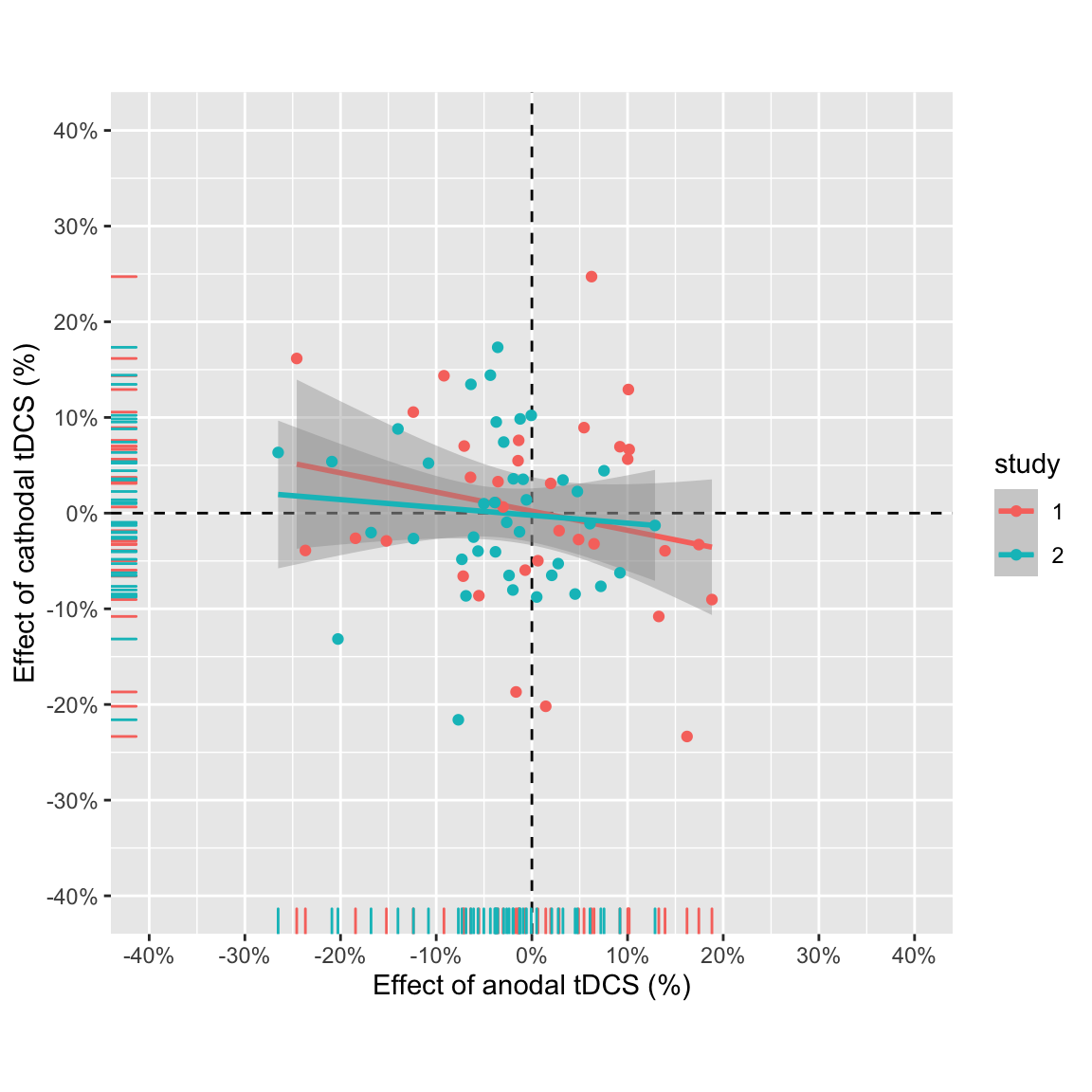
Effect of anodal vs. effect of cathodal pooled across studies
The negative correlation is larger in study 1, and the data points from study 1 have a bigger spread. But overall it doesn’t look very convincing still.
Statistics
Partial correlation between anodal and cathodal AB magnitude change score (tDCS - baseline), attempting to adjust for session order:
pcorr_anodal_cathodal(filter(ABmagChange_pooled, change == "tDCS - baseline")) %>%
kable(digits = 3, caption = "Pooled data from studies 1 and 2: Partial correlation anodal vs. cathodal")| change | r | tval | df | pvalue |
|---|---|---|---|---|
| tDCS - baseline | -0.176 | -1.509 | 71 | 0.136 |
Zero-order correlation:
tidy(cor.test(
  pull(filter(ABmagChange_pooled, stimulation == "anodal", measure == "AB.magnitude", change == "tDCS - baseline"), change.score),
  pull(filter(ABmagChange_pooled, stimulation == "cathodal", measure == "AB.magnitude", change == "tDCS - baseline"), change.score),
  method = "pearson")) %>%
kable(., digits = 3, caption = "Pooled data from studies 1 and 2: Zero-order correlation anodal vs. cathodal")| estimate | statistic | p.value | parameter | conf.low | conf.high | method | alternative |
|---|---|---|---|---|---|---|---|
| -0.158 | -1.354 | 0.18 | 72 | -0.373 | 0.074 | Pearson’s product-moment correlation | two.sided |
Bayes factor:
extractBF(correlationBF(
  pull(filter(ABmagChange_pooled, stimulation == "anodal", measure == "AB.magnitude", change == "tDCS - baseline"), change.score),
  pull(filter(ABmagChange_pooled, stimulation == "cathodal", measure == "AB.magnitude", change == "tDCS - baseline"), change.score))) %>%
  select(bf) %>% # keep only the Bayes Factor
kable(digits = 3, caption = "Pooled data from studies 1 and 2: Bayesian correlation")| bf | |
|---|---|
| Alt., r=0.333 | 0.613 |
Neither correlation is significant. The Bayes factor favors the null, but only slightly, and less so than in study 2.
Meta-analysis
For a more orthodox look on the pooled effect from both studies, let’s perform a meta-analysis of the correlation coefficients.
First, create a new data frame with all the information:
df_meta <- tibble(authors = c("London & Slagter","Reteig et al."), year = c(2021,2021),
                  ni = c(n_study1_pc, n_study2_pc),
                  ri = c(r_study1, r_study2))
kable(df_meta)| authors | year | ni | ri |
|---|---|---|---|
| London & Slagter | 2021 | 33 | -0.4453648 |
| Reteig et al. | 2021 | 39 | 0.0209995 |
- ni is the sample size in each study
- ri is the correlation coefficient (Pearson’s r)
We’ll specify the meta-analysis as a fixed effects model, as both studies were highly similar and from the same population (same lab, same university student sample). This does mean our inferences are limited to this particular set of two studies, but that’s also what we want to know in this case (“how large is the effect when we pool both studies”), not necessarily “how large is the true effect in the population” (which would be a random-effects meta-analysis).
res <- rma(ri = ri, ni = ni, data = df_meta,
           measure = "ZCOR", method = "FE", # Fisher-z tranform of r values, fixed effects method
           slab = paste(authors, year, sep = ", ")) # add study info to "res" list
res
## ## Fixed-Effects Model (k = 2) ## ## I^2 (total heterogeneity / total variability): 75.55% ## H^2 (total variability / sampling variability): 4.09 ## ## Test for Heterogeneity: ## Q(df = 1) = 4.0894, p-val = 0.0432 ## ## Model Results: ## ## estimate se zval pval ci.lb ci.ub ## -0.2062 0.1231 -1.6754 0.0939 -0.4475 0.0350 . ## ## --- ## Signif. codes: 0 '***' 0.001 '**' 0.01 '*' 0.05 '.' 0.1 ' ' 1
The overall effect is not significant: p = 0.094.
The effect size and confidence intervals printed above are z-values, as the meta-analysis was performed on Fisher’s r-to-z transformed correlation coefficients. Now we transform them back to r-values:
kable(predict(res, transf = transf.ztor))| pred | ci.lb | ci.ub | |
|---|---|---|---|
| -0.2033526 | -0.4198272 | 0.0350132 |
- pred is the correlation coefficient r
- ci.lb and ci.ub are the upper and lower bounds of the confidence interval around r
We can also visualize all of this in a forest plot:
forest(res, transf = transf.ztor)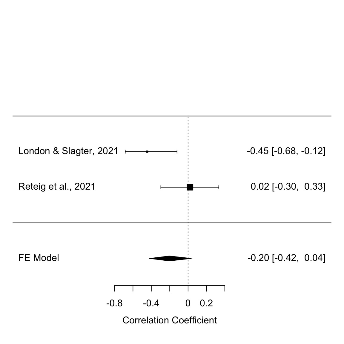
Fixed-effects meta-analysis of the anodal vs. cathodal correlation in study 1 and 2
This shows the r-values (squares) and CIs (error bars) of the individual studies, as well as the meta-analytic effect size (middle of the diamond) and CI (ends of the diamond). The CIs of the meta-analytic effect just overlap zero, so the overall effect is not significant.
Prediction intervals
To evaluate whether the result observed in study 2 is consistent with study 1, we can construct a prediction interval. A prediction interval contains the range of correlation coefficients we can expect to see in study 2, based on the original correlation in study 1, and the sample sizes of both study 1 and 2.
If the original study were replicated 100 times, 95 of the observed correlation coefficients would fall within the 95% prediction interval. Note that this is different from a confidence interval, which quantifies uncertainty about the (unknown) true correlation in the population (95 out of every hundred 95% CIs contain the true population parameter).
pi.r(r = r_study1, n = n_study1_pc, rep.n = n_study2_pc)## ## Original study: r = -0.45, N = 33, 95% CI[-0.68, -0.12] ## Replication study: N = 39 ## Prediction interval: 95% PI[-0.82,-0.05]. ## ## ## Interpretation: ## The original correlation is -0.45 - with a prediction interval 95% PI[-0.82, -0.05] based a replication sample size of N = 39. If the replication correlation differs from the original correlation only due to sampling error, there is a 95% chance the replication result will fall in this interval. If the replication correlation falls outside of this range, factors beyond sampling error are likely also responsible for the difference.
The observed correlation in study 2 (r = 0.02) falls outside the 95% PI. Therefore, the results of study 2 are not consistent with study 1, so we could conclude that study 2 was a succesful replication.
However, the 95% PI is so wide that almost any negative correlation of a realistic size would fall inside it. So above all it illustrates that we cannot draw strong conclusions based on the results of either study.
Bayes Factors with informed priors
bf_study2 <- extractBF(correlationBF(
  pull(filter(ABmagChange_study2, stimulation == "anodal", measure == "AB.magnitude", change == "tDCS - baseline"), change.score),
  pull(filter(ABmagChange_study2, stimulation == "cathodal", measure == "AB.magnitude", change == "tDCS - baseline"), change.score))) %>%
  select(bf) # keep only the Bayes Factor

kable(bf_study2)| bf | |
|---|---|
| Alt., r=0.333 | 0.3969199 |
One-sided
The default Bayes Factor uses a prior that assigns equal weight to positive and negative effect sizes (correlation coefficients in our case). However, we can also “fold” all the prior mass to one side, thereby effectively testing a directional hypothesis.
In our case, based on study 1, we expect a negative correlation, so we evaluate the prior only over negative effect sizes (-1 to 0)
bf_one_sided <- extractBF(correlationBF(
  pull(filter(ABmagChange_study2, stimulation == "anodal", measure == "AB.magnitude", change == "tDCS - baseline"), change.score),
  pull(filter(ABmagChange_study2, stimulation == "cathodal", measure == "AB.magnitude", change == "tDCS - baseline"), change.score),
  nullInterval = c(-1,0))) %>%
  select(bf) # keep only the Bayes Factor

kable(bf_one_sided)| bf | |
|---|---|
| Alt., r=0.333 -1<rho<0 | 0.5446767 |
| Alt., r=0.333 !(-1<rho<0) | 0.2491474 |
This Bayes Factor still provides more evidence for the null than for the alternative, but does provide less evidence for the null (BF01 = 1 / 0.54 = 1.84) than the regular Bayes Factor (BF01 = 1 / 0.4 = 2.52)
“Replication Bayes Factor”
While a default Bayes factor adresses the question (“Is there more evidence that the effect is absent (H0) vs. present (H1), this Bayes factors adresses the question (”Is there more evidence that the effect is absent (the “skeptic’s hypothesis”) vs. similar to what was found before ( the “proponent’s hypothesis”). The “replication Bayes factor” adresses this latter question by using the posterior of study 1 as a prior in the analysis of study 2, i.e. as the proponent’s hypothesis.
This Bayes factor was proposed by Wagenmakers, Verhagen & Ly (2016)2 and is computed using their provided code. Note that it does not “directly” compute a Bayesian correlation, but uses the effect sizes (partial correlations) from both studies.
bf0RStudy1 <- 1/repBfR0(nOri = n_study1_pc, rOri = r_study1,
                        nRep = n_study2_pc, rRep = r_study2)
bf0RStudy1
## [1] 9.657519
This BF expresses that the data are 9.66 times more likely under the skeptic’s hypothesis, than under the proponent’s hypothesis.
Equivalence tests
Equivalence tests allow you to test for the absence of an effect of a specific size. Usually this is the smallest effect size of interest (the SESOI). We’ll use three different specifications of the SESOI.
Small telescopes
The “Small Telescopes” approach (Simonsohn, 2015)3 suggests that the SESOI should be the effect size the original study had 33% power to detect, the idea being that anything smaller than that could not have been properly investigated in the original study in the first place (as the odds were already stacked 2:1 against finding the effect).
small_telescopes <- pwr.r.test(n_study1_pc, power = 0.33) # r value with 33% power in study 1
TOSTr(n = n_study2_pc, r = r_study2,
      high_eqbound_r = small_telescopes$r,
      low_eqbound_r = -small_telescopes$r, alpha = 0.05) # equivalence test
## TOST results: ## p-value lower bound: 0.038 ## p-value upper bound: 0.065 ## ## Equivalence bounds (r): ## low eqbound: -0.2673 ## high eqbound: 0.2673 ## ## TOST confidence interval: ## lower bound 90% CI: -0.248 ## upper bound 90% CI: 0.287 ## ## NHST confidence interval: ## lower bound 95% CI: -0.296 ## upper bound 95% CI: 0.334 ## ## Equivalence Test Result: ## The equivalence test was non-significant, p = 0.0645, given equivalence bounds of -0.267 and 0.267 and an alpha of 0.05.
## ## ## Null Hypothesis Test Result: ## The null hypothesis test was non-significant, p = 0.899, given an alpha of 0.05.
## ## ## Based on the equivalence test and the null-hypothesis test combined, we can conclude that the observed effect is statistically not different from zero and statistically not equivalent to zero.
## 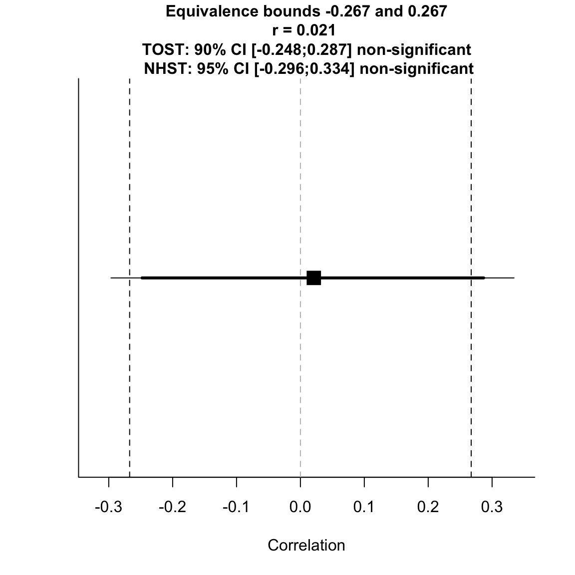
test for equivalence to 33% power effect size
The overall equivalence test is not significant, so we cannot conclude that the effect is smaller than the SESOI. However, given the original study found a negative effect, it makes sense to only look at the lower equivalence bound. The results of this inferiority test is in fact significant, so we can reject the hypothesis that the effect size is at least that negative.
Critical effect size
Others (e.g. in the paper accompanying the R package for equivalence test, by Lakens et al. (2018)4) argue that a more appropriate SESOI would be the smallest effect size that would still be significant in the original study. This usually corresponds to the effect size the study had 50% power to detect.
First we derive the critical r-value for the original sample size (function below from https://www.researchgate.net/post/What_is_the_formula_to_calculate_the_critical_value_of_correlation).
critical.r <- function(n, alpha = .05 ) {
    df <- n - 2
    critical.t <- qt( alpha/2, df, lower.tail = F )
    critical.r <- sqrt( (critical.t^2) / ( (critical.t^2) + df ) )
    return( critical.r )
}
critical.r(n_study1_pc)
## [1] 0.3439573
TOSTr(n = n_study2_pc, r = r_study2,
      high_eqbound_r = critical.r(n_study1_pc),
      low_eqbound_r = -critical.r(n_study1_pc),
      alpha = 0.05)
## TOST results: ## p-value lower bound: 0.011 ## p-value upper bound: 0.021 ## ## Equivalence bounds (r): ## low eqbound: -0.344 ## high eqbound: 0.344 ## ## TOST confidence interval: ## lower bound 90% CI: -0.248 ## upper bound 90% CI: 0.287 ## ## NHST confidence interval: ## lower bound 95% CI: -0.296 ## upper bound 95% CI: 0.334 ## ## Equivalence Test Result: ## The equivalence test was significant, p = 0.0214, given equivalence bounds of -0.344 and 0.344 and an alpha of 0.05.
## ## ## Null Hypothesis Test Result: ## The null hypothesis test was non-significant, p = 0.899, given an alpha of 0.05.
## ## ## Based on the equivalence test and the null-hypothesis test combined, we can conclude that the observed effect is statistically not different from zero and statistically equivalent to zero.
## 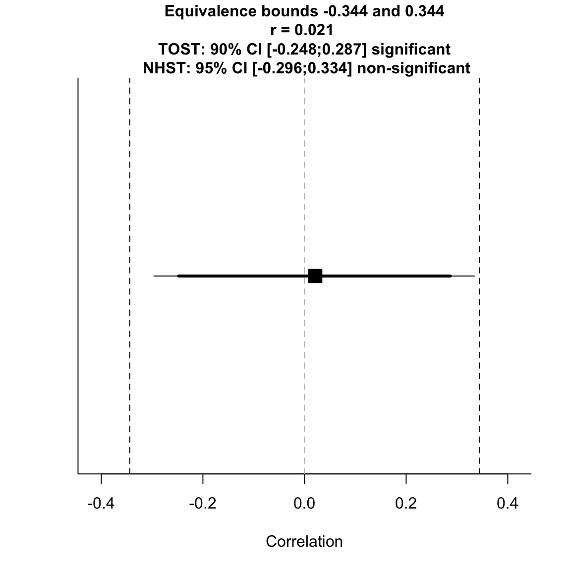
test for equivalence to critical effect size
When we specify the SESOI like this, the CIs do fall within both equivalence bounds.
Original effect size
Finally, we can also take the original effect size as the SESOI.
TOSTr(n = n_study2_pc, r = r_study2, high_eqbound_r = -r_study1, low_eqbound_r = r_study1, alpha = 0.05)## TOST results: ## p-value lower bound: 0.001 ## p-value upper bound: 0.003 ## ## Equivalence bounds (r): ## low eqbound: -0.4454 ## high eqbound: 0.4454 ## ## TOST confidence interval: ## lower bound 90% CI: -0.248 ## upper bound 90% CI: 0.287 ## ## NHST confidence interval: ## lower bound 95% CI: -0.296 ## upper bound 95% CI: 0.334 ## ## Equivalence Test Result: ## The equivalence test was significant, p = 0.003, given equivalence bounds of -0.445 and 0.445 and an alpha of 0.05.
## ## ## Null Hypothesis Test Result: ## The null hypothesis test was non-significant, p = 0.899, given an alpha of 0.05.
## ## ## Based on the equivalence test and the null-hypothesis test combined, we can conclude that the observed effect is statistically not different from zero and statistically equivalent to zero.
## 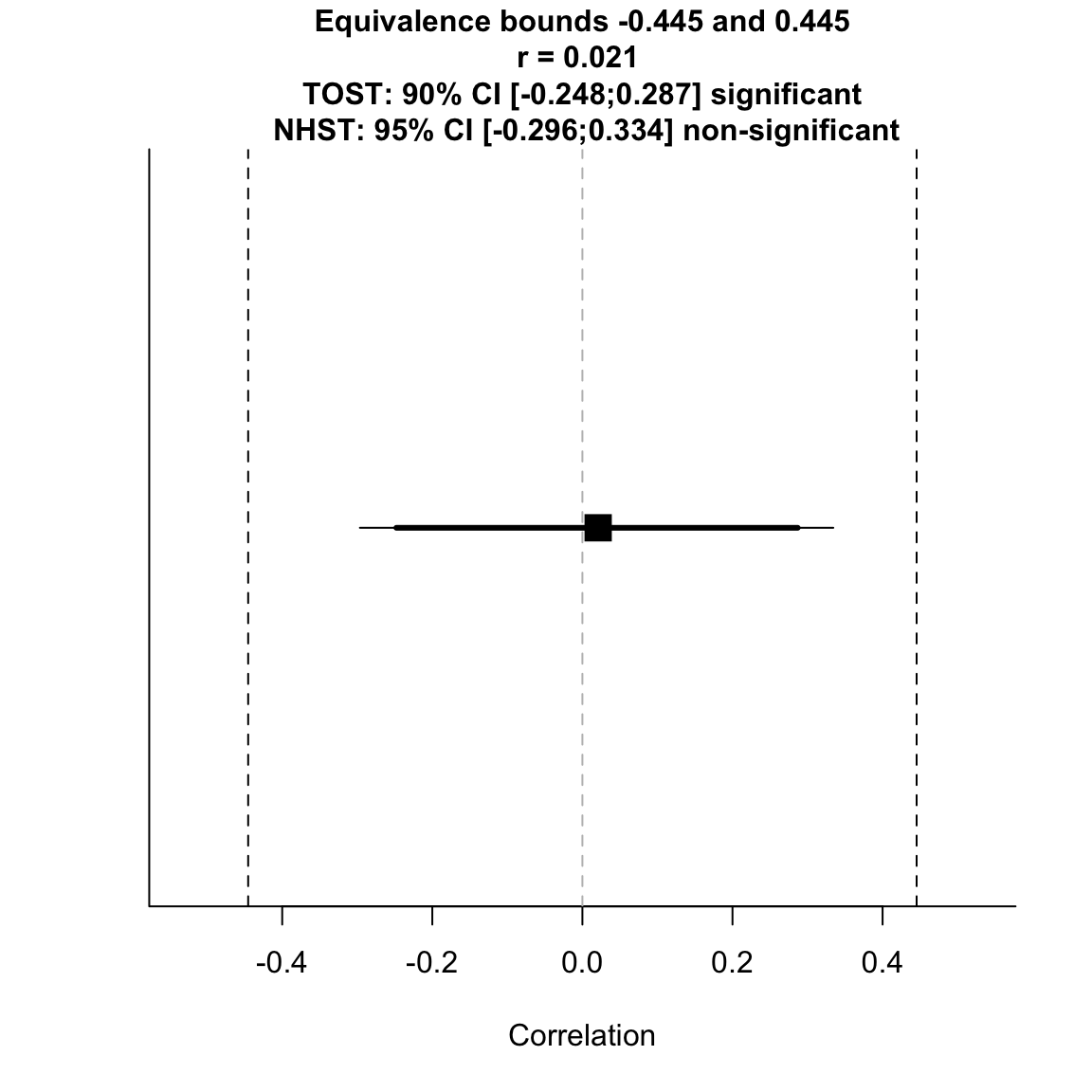
test for equivalence to original effect size
This is the least stringent criterion, so naturally this test is also significant, meaning that based on study 2 we can reject the presence of a correlation at least as large as in study 1.
However, given that the original correlation was not very precisely estimated (the confidence intervals were very wide), this is not really a reasonable SESOI.
London, R. E., & Slagter, H. A. (2021). No Effect of Transcranial Direct Current Stimulation over Left Dorsolateral Prefrontal Cortex on Temporal Attention. Journal of Cognitive Neuroscience, 33(4), 756–768. doi: 10.1162/jocn_a_01679↩︎
Wagenmakers, E. J., Verhagen, J., & Ly, A. (2016). How to quantify the evidence for the absence of a correlation. Behavior Research Methods, 48(2), 413-426. doi: 10.3758/s13428-015-0593-0↩︎
Simonsohn, U. (2015). Small telescopes: Detectability and the evaluation of replication results. Psychological Science, 26(5),, 1–11. doi: 10.1177/0956797614567341↩︎
Lakens, D., Scheel, A. M., & Isager, P. M. (2018). Equivalence Testing for Psychological Research: A Tutorial. Advances in Methods and Practices in Psychological Science, 1(2), 259–269. doi: 10.1177/2515245918770963↩︎