Setup environment
# Load packages
library(tidyverse)  # importing, transforming, and visualizing data frames
## ── Attaching packages ─────────────────────────────────────── tidyverse 1.3.0 ──## ✓ ggplot2 3.3.3 ✓ purrr 0.3.4
## ✓ tibble 3.0.6 ✓ dplyr 1.0.4
## ✓ tidyr 1.1.2 ✓ stringr 1.4.0
## ✓ readr 1.4.0 ✓ forcats 0.5.1## ── Conflicts ────────────────────────────────────────── tidyverse_conflicts() ──
## x dplyr::filter() masks stats::filter()
## x dplyr::lag() masks stats::lag()library(here) # (relative) file paths## here() starts at /Users/leonreteig/AB-tDCSlibrary(knitr) # R notebook output
library(scales) # Percentage axis labels ##
## Attaching package: 'scales'## The following object is masked from 'package:purrr':
##
## discard## The following object is masked from 'package:readr':
##
## col_factorlibrary(ggm) # partial correlations
library(BayesFactor) # Bayesian statistics## Loading required package: coda## Loading required package: Matrix##
## Attaching package: 'Matrix'## The following objects are masked from 'package:tidyr':
##
## expand, pack, unpack## ************
## Welcome to BayesFactor 0.9.12-4.2. If you have questions, please contact Richard Morey (richarddmorey@gmail.com).
##
## Type BFManual() to open the manual.
## ************library(knitrhooks) # printing in rmarkdown outputs
output_max_height()
# Source functions
source(here("src", "func", "behavioral_analysis.R")) # loading data and calculating measures
knitr::read_chunk(here("src", "func", "behavioral_analysis.R")) # display code from file in this notebook
load_data_path <- here("src","func","load_data.Rmd") # for rerunning and displaying
source(here("src", "lib", "corr_change_baseline.R")) # variance test / baseline vs. change-from-baseline correlation print(sessionInfo())## R version 3.6.2 (2019-12-12) ## Platform: x86_64-apple-darwin15.6.0 (64-bit) ## Running under: macOS 10.16 ## ## Matrix products: default ## BLAS: /Library/Frameworks/R.framework/Versions/3.6/Resources/lib/libRblas.0.dylib ## LAPACK: /Library/Frameworks/R.framework/Versions/3.6/Resources/lib/libRlapack.dylib ## ## locale: ## [1] en_US.UTF-8/en_US.UTF-8/en_US.UTF-8/C/en_US.UTF-8/en_US.UTF-8 ## ## attached base packages: ## [1] stats graphics grDevices datasets utils methods base ## ## other attached packages: ## [1] knitrhooks_0.0.4 BayesFactor_0.9.12-4.2 Matrix_1.3-2 ## [4] coda_0.19-4 ggm_2.5 scales_1.1.1 ## [7] knitr_1.31 here_1.0.1 forcats_0.5.1 ## [10] stringr_1.4.0 dplyr_1.0.4 purrr_0.3.4 ## [13] readr_1.4.0 tidyr_1.1.2 tibble_3.0.6 ## [16] ggplot2_3.3.3 tidyverse_1.3.0 ## ## loaded via a namespace (and not attached): ## [1] Rcpp_1.0.6 lubridate_1.7.9.2 mvtnorm_1.1-1 lattice_0.20-41 ## [5] gtools_3.8.2 assertthat_0.2.1 rprojroot_2.0.2 digest_0.6.27 ## [9] R6_2.5.0 cellranger_1.1.0 backports_1.2.1 MatrixModels_0.5-0 ## [13] reprex_1.0.0 evaluate_0.14 httr_1.4.2 pillar_1.4.7 ## [17] rlang_0.4.10 readxl_1.3.1 rstudioapi_0.13 jquerylib_0.1.4 ## [21] rmarkdown_2.11 igraph_1.2.6 munsell_0.5.0 broom_0.7.4.9000 ## [25] compiler_3.6.2 modelr_0.1.8 xfun_0.21 pkgconfig_2.0.3 ## [29] htmltools_0.5.1.1 tidyselect_1.1.0 bookdown_0.21 crayon_1.4.1 ## [33] dbplyr_2.1.0 withr_2.4.1 grid_3.6.2 jsonlite_1.7.2 ## [37] gtable_0.3.0 lifecycle_1.0.0 DBI_1.1.1 magrittr_2.0.1 ## [41] rmdformats_1.0.2 cli_2.3.0 stringi_1.5.3 pbapply_1.4-3 ## [45] renv_0.12.5-72 fs_1.5.0 xml2_1.3.2 ellipsis_0.3.1 ## [49] generics_0.1.0 vctrs_0.3.6 tools_3.6.2 glue_1.4.2 ## [53] hms_1.0.0 parallel_3.6.2 yaml_2.2.1 colorspace_2.0-0 ## [57] rvest_0.3.6 haven_2.3.1
Load task data
Study 2
The following participants are excluded from further analysis at this point, because of incomplete data:
S03,S14,S29,S38,S43,S46: their T1 performance in session 1 was less than 63% correct, so they were not invited back. This cutoff was determined based on a separate pilot study with 10 participants. It is two standard deviations below the mean of that sample.S25has no data for session 2, as they stopped responding to requests for scheduling the sessionS31was excluded as a precaution after session 1, as they developed a severe headache and we could not rule out the possibility this was related to the tDCS
dataDir_study2 <- here("data") # root folder with AB task data
subs_incomplete <- c("S03", "S14", "S25", "S29", "S31", "S38", "S43", "S46") # don't try to load data from these participants
df_study2 <- load_data_study2(dataDir_study2, subs_incomplete) %>%
  filter(complete.cases(.)) %>% # discard rows with data from incomplete subjects
   # recode first.session ("anodal" or "cathodal") to session.order ("anodal first", "cathodal first")
  mutate(first.session = parse_factor(paste(first.session, "first"),
                                      levels = c("anodal first", "cathodal first"))) %>%
  rename(session.order = first.session)
n_study2 <- n_distinct(df_study2$subject) # number of subjects in study 2kable(head(df_study2,13), digits = 1, caption = "Data frame for study 2")| subject | session.order | stimulation | block | lag | trials | T1 | T2 | T2.given.T1 |
|---|---|---|---|---|---|---|---|---|
| S01 | anodal first | anodal | pre | 3 | 118 | 0.8 | 0.4 | 0.4 |
| S01 | anodal first | anodal | pre | 8 | 60 | 0.8 | 0.8 | 0.8 |
| S01 | anodal first | anodal | tDCS | 3 | 126 | 0.8 | 0.3 | 0.3 |
| S01 | anodal first | anodal | tDCS | 8 | 65 | 0.8 | 0.7 | 0.7 |
| S01 | anodal first | anodal | post | 3 | 122 | 0.8 | 0.2 | 0.3 |
| S01 | anodal first | anodal | post | 8 | 61 | 0.7 | 0.7 | 0.7 |
| S01 | anodal first | cathodal | pre | 3 | 116 | 0.8 | 0.4 | 0.4 |
| S01 | anodal first | cathodal | pre | 8 | 60 | 0.7 | 0.8 | 0.8 |
| S01 | anodal first | cathodal | tDCS | 3 | 129 | 0.7 | 0.4 | 0.4 |
| S01 | anodal first | cathodal | tDCS | 8 | 64 | 0.7 | 0.8 | 0.9 |
| S01 | anodal first | cathodal | post | 3 | 128 | 0.6 | 0.4 | 0.4 |
| S01 | anodal first | cathodal | post | 8 | 62 | 0.7 | 0.8 | 0.8 |
| S02 | cathodal first | anodal | pre | 3 | 124 | 1.0 | 0.8 | 0.8 |
The data has the following columns:
- subject: Participant ID, e.g.
S01,S12 - session.order: Whether participant received
anodalorcathodaltDCS in the first session (anodal_firstvs.cathodal_first). - stimulation: Whether participant received
anodalorcathodaltDCS - block: Whether data is before (
pre), during (tDCS) or after (post`) tDCS - lag: Whether T2 followed T1 after two distractors (lag
3) or after 7 distractors (lag8) - trials: Number of trials per lag that the participant completed in this block
- T1: Proportion of trials (out of
trials) in which T1 was identified correctly - T2: Proportion of trials (out of
trials) in which T2 was identified correctly - T2.given.T1: Proportion of trials which T2 was identified correctly, out of the trials in which T1 was idenitified correctly (T2|T1).
The number of trials vary from person-to-person, as some completed more trials in a 20-minute block than others (because responses were self-paced):
df_study2 %>%
  group_by(lag) %>%
  summarise_at(vars(trials), funs(mean, min, max, sd)) %>%
  kable(caption = "Descriptive statistics for trial counts per lag", digits = 0)
## Warning: `funs()` was deprecated in dplyr 0.8.0.
## Please use a list of either functions or lambdas:
##
## # Simple named list:
## list(mean = mean, median = median)
##
## # Auto named with `tibble::lst()`:
## tibble::lst(mean, median)
##
## # Using lambdas
## list(~ mean(., trim = .2), ~ median(., na.rm = TRUE))| lag | mean | min | max | sd |
|---|---|---|---|---|
| 3 | 130 | 78 | 163 | 17 |
| 8 | 65 | 39 | 87 | 9 |
Study 1
These data were used for statistical analysis in London & Slagter (2021)1, and were processed by the lead author:
dataPath_study1 <- here("data","AB-tDCS_study1.txt")
data_study1_fromDisk <- read.table(dataPath_study1, header = TRUE, dec = ",")
glimpse(data_study1_fromDisk)
## Rows: 34 ## Columns: 120 ## $ SD_T10.3313, 0.0289, -0.8027, -0.5381, -2.… ## $ MeanBLT1Acc 0.8800, 0.8600, 0.8050, 0.8225, 0.665… ## $ First_Session 1, 2, 1, 1, 2, 1, 2, 1, 2, 2, 1, 2, 1… ## $ fileno pp4, pp6, pp7, pp9, pp10, pp11, pp12,… ## $ AB_HighLow 2, 1, 2, 1, 1, 1, 1, 1, 2, 1, 1, 2, 1… ## $ vb_T1_2_NP 0.925, 0.875, 0.825, 0.625, 0.650, 0.… ## $ vb_T1_4_NP 0.800, 0.825, 0.825, 0.825, 0.675, 0.… ## $ vb_T1_10_NP 0.925, 0.925, 0.800, 0.775, 0.825, 0.… ## $ vb_T1_4_P 0.850, 0.900, 0.825, 0.775, 0.625, 0.… ## $ vb_T1_10_P 0.825, 0.900, 0.775, 0.825, 0.625, 0.… ## $ vb_NB_2_NP 0.1351, 0.3429, 0.3636, 0.3600, 0.346… ## $ vb_NB_4_NP 0.3125, 0.5455, 0.5455, 0.3030, 0.296… ## $ vb_NB_10_NP 0.8378, 0.8108, 0.9688, 0.6129, 0.727… ## $ vb_NB_4_P 0.2941, 0.5278, 0.6061, 0.3226, 0.520… ## $ vb_NB_10_P 0.8485, 0.7778, 0.9032, 0.8182, 0.680… ## $ VB_AB 0.7027, 0.4680, 0.6051, 0.2529, 0.381… ## $ VB_REC 0.5253, 0.2654, 0.4233, 0.3099, 0.431… ## $ VB_PE -0.0184, -0.0177, 0.0606, 0.0196, 0.2… ## $ tb_T1_2_NP 0.775, 0.875, 0.675, 0.725, 0.475, 0.… ## $ tb_T1_4_NP 0.825, 0.825, 0.700, 0.750, 0.675, 0.… ## $ tb_T1_10_NP 0.875, 0.900, 0.700, 0.825, 0.500, 0.… ## $ tb_T1_4_P 0.875, 0.800, 0.700, 0.775, 0.650, 0.… ## $ tb_T1_10_P 0.850, 0.925, 0.800, 0.825, 0.625, 0.… ## $ tb_NB_2_NP 0.1290, 0.5143, 0.2222, 0.0690, 0.315… ## $ tb_NB_4_NP 0.3333, 0.5455, 0.6071, 0.1333, 0.370… ## $ tb_NB_10_NP 0.8286, 0.8611, 0.8571, 0.5152, 0.850… ## $ tb_NB_4_P 0.3143, 0.6250, 0.5357, 0.4839, 0.538… ## $ tb_NB_10_P 0.8529, 0.7568, 0.9375, 0.6667, 0.680… ## $ TB_AB 0.6995, 0.3468, 0.6349, 0.4462, 0.534… ## $ TB_REC 0.4952, 0.3157, 0.2500, 0.3818, 0.479… ## $ TB_PE -0.0190, 0.0795, -0.0714, 0.3505, 0.1… ## $ nb_T1_2_NP 0.850, 0.850, 0.650, 0.725, 0.675, 0.… ## $ nb_T1_4_NP 0.800, 0.850, 0.725, 0.675, 0.575, 0.… ## $ nb_T1_10_NP 0.925, 0.825, 0.750, 0.850, 0.725, 0.… ## $ nb_T1_4_P 0.850, 0.900, 0.675, 0.750, 0.875, 0.… ## $ nb_T1_10_P 0.900, 0.825, 0.750, 0.800, 0.550, 0.… ## $ nb_NB_2_NP 0.0588, 0.4412, 0.4615, 0.1034, 0.296… ## $ nb_NB_4_NP 0.0938, 0.4412, 0.2414, 0.1481, 0.478… ## $ nb_NB_10_NP 0.8649, 0.7576, 0.9667, 0.6765, 0.896… ## $ nb_NB_4_P 0.4118, 0.7222, 0.4815, 0.3667, 0.685… ## $ nb_NB_10_P 0.8333, 0.8485, 0.8333, 0.7188, 0.818… ## $ NB_AB 0.8060, 0.3164, 0.5051, 0.5730, 0.600… ## $ NB_REC 0.7711, 0.3164, 0.7253, 0.5283, 0.418… ## $ NB_PE 0.3180, 0.2810, 0.2401, 0.2185, 0.207… ## $ vd_T1_2_NP 0.925, 0.875, 0.800, 0.850, 0.575, 0.… ## $ vd_T1_4_NP 0.850, 0.825, 0.825, 0.925, 0.700, 0.… ## $ vd_T1_10_NP 0.850, 0.900, 0.825, 0.925, 0.750, 0.… ## $ vd_T1_4_P 0.925, 0.775, 0.825, 0.750, 0.650, 0.… ## $ vd_T1_10_P 0.925, 0.800, 0.725, 0.950, 0.575, 0.… ## $ vd_NB_2_NP 0.0541, 0.2857, 0.3125, 0.1765, 0.173… ## $ vd_NB_4_NP 0.2941, 0.4848, 0.4545, 0.2432, 0.428… ## $ vd_NB_10_NP 1.0000, 0.6667, 0.9394, 0.7838, 0.766… ## $ vd_NB_4_P 0.5135, 0.6774, 0.4848, 0.5000, 0.500… ## $ vd_NB_10_P 0.8919, 0.8125, 0.9310, 0.8421, 0.608… ## $ VD_AB 0.9459, 0.3810, 0.6269, 0.6073, 0.592… ## $ VD_REC 0.7059, 0.1818, 0.4848, 0.5405, 0.338… ## $ VD_PE 0.2194, 0.1926, 0.0303, 0.2568, 0.071… ## $ td_T1_2_NP 0.950, 0.775, 0.625, 0.775, 0.525, 0.… ## $ td_T1_4_NP 0.975, 0.800, 0.800, 0.750, 0.625, 0.… ## $ td_T1_10_NP 0.975, 0.900, 0.800, 0.850, 0.575, 0.… ## $ td_T1_4_P 0.875, 0.800, 0.800, 0.800, 0.600, 0.… ## $ td_T1_10_P 0.875, 0.800, 0.850, 0.700, 0.525, 0.… ## $ td_NB_2_NP 0.1579, 0.3226, 0.5200, 0.1290, 0.142… ## $ td_NB_4_NP 0.4615, 0.4375, 0.3750, 0.2333, 0.320… ## $ td_NB_10_NP 0.9487, 0.6944, 0.9375, 0.6471, 0.826… ## $ td_NB_4_P 0.4571, 0.3750, 0.5625, 0.4063, 0.583… ## $ td_NB_10_P 0.8857, 0.6875, 0.8529, 0.7143, 0.666… ## $ TD_AB 0.7908, 0.3719, 0.4175, 0.5180, 0.683… ## $ TD_REC 0.4872, 0.2569, 0.5625, 0.4137, 0.506… ## $ TD_PE -0.0044, -0.0625, 0.1875, 0.1729, 0.2… ## $ nd_T1_2_NP 0.700, 0.800, 0.650, 0.775, 0.425, 0.… ## $ nd_T1_4_NP 0.850, 0.850, 0.725, 0.850, 0.650, 0.… ## $ nd_T1_10_NP 0.800, 0.825, 0.800, 0.850, 0.600, 0.… ## $ nd_T1_4_P 0.850, 0.800, 0.775, 0.775, 0.725, 0.… ## $ nd_T1_10_P 0.850, 0.750, 0.800, 0.850, 0.675, 0.… ## $ nd_NB_2_NP 0.0000, 0.2188, 0.2692, 0.0968, 0.235… ## $ nd_NB_4_NP 0.3824, 0.5000, 0.5172, 0.2353, 0.384… ## $ nd_NB_10_NP 0.8750, 0.5758, 0.8125, 0.7941, 0.708… ## $ nd_NB_4_P 0.4118, 0.5000, 0.5806, 0.5484, 0.482… ## $ nd_NB_10_P 0.9118, 0.7667, 0.8438, 0.8235, 0.629… ## $ ND_AB 0.8750, 0.3570, 0.5433, 0.6973, 0.473… ## $ ND_REC 0.4926, 0.0758, 0.2953, 0.5588, 0.323… ## $ ND_PE 0.0294, 0.0000, 0.0634, 0.3131, 0.098… ## $ AnoMinBl_Lag2_NP -0.01, 0.17, -0.14, -0.29, -0.03, 0.0… ## $ AnoMinBl_Lag10_NP -0.01, 0.05, -0.11, -0.10, 0.12, -0.0… ## $ CathoMinBl_Lag2_NP 0.10, 0.04, 0.21, -0.05, -0.03, 0.09,… ## $ CathoMinBl_Lag10_NP -0.05, 0.03, 0.00, -0.14, 0.06, 0.00,… ## $ Tijdens_AnoMinBl_Lag2_NP -0.01, 0.17, -0.14, -0.29, -0.03, 0.0… ## $ Tijdens_AnoMinBl_Lag10_NP -0.01, 0.05, -0.11, -0.10, 0.12, -0.0… ## $ Tijdens_CathoMinBl_Lag2_NP 0.10, 0.04, 0.21, -0.05, -0.03, 0.09,… ## $ Tijdens_CathoMinBl_Lag10_NP -0.05, 0.03, 0.00, -0.14, 0.06, 0.00,… ## $ Tijdens_AnoMinBL_AB 0.00, -0.12, 0.03, 0.19, 0.15, -0.08,… ## $ Tijdens_CathoMinBL_AB -0.16, -0.01, -0.21, -0.09, 0.09, -0.… ## $ Na_AnoMinBL_AB 0.10, -0.15, -0.10, 0.32, 0.22, -0.04… ## $ Na_CathoMinBL_AB -0.07, -0.02, -0.08, 0.09, -0.12, -0.… ## $ Tijdens_AnoMinBL_PE 0.00, 0.10, -0.13, 0.33, -0.06, -0.06… ## $ Tijdens_CathoMinBL_PE -0.22, -0.26, 0.16, -0.08, 0.19, -0.0… ## $ Na_CathoMinBL_PE -0.19, -0.19, 0.03, 0.06, 0.03, 0.31,… ## $ Na_AnoMinBL_PE 0.34, 0.30, 0.18, 0.20, -0.02, 0.06, … ## $ Tijdens_AnoMinBL_REC -0.03, 0.05, -0.17, 0.07, 0.05, 0.07,… ## $ Tijdens_CathoMinBL_REC -0.22, 0.08, 0.08, -0.13, 0.17, -0.03… ## $ Na_CathoMinBL_REC -0.21, -0.11, -0.19, 0.02, -0.01, 0.1… ## $ Na_AnoMinBL_REC 0.25, 0.05, 0.30, 0.22, -0.01, 0.13, … ## $ T1_Lag2_Tijdens_Ano_Min_BL_NP -0.15, 0.00, -0.15, 0.10, -0.18, 0.00… ## $ T1_Lag2_Tijdens_Catho_Min_BL_NP 0.02, -0.10, -0.18, -0.08, -0.05, -0.… ## $ T1_Lag2_Na_Ano_Min_BL_NP -0.08, -0.03, -0.18, 0.10, 0.03, -0.1… ## $ T1_Lag2_Na_Catho_Min_BL_NP -0.23, -0.08, -0.15, -0.08, -0.15, -0… ## $ T1_Lag4_Tijdens_Ano_Min_BL_NP 0.02, 0.00, -0.13, -0.08, 0.00, 0.05,… ## $ T1_Lag4_Tijdens_Catho_Min_BL_NP 0.13, -0.02, -0.02, -0.18, -0.08, 0.0… ## $ T1_Lag4_Na_Catho_Min_BL_NP 0.00, 0.03, -0.10, -0.08, -0.05, 0.13… ## $ T1_Lag4_Na_Ano_Min_BL_NP 0.00, 0.03, -0.10, -0.15, -0.10, 0.02… ## $ Mean_BL_PE 0.10, 0.09, 0.05, 0.14, 0.15, -0.13, … ## $ ZVB_AB 0.72613, -0.71847, 0.12559, -2.04185,… ## $ ZTB_AB 0.97738, -1.74477, 0.47867, -0.97793,… ## $ ZNB_AB 1.24043, -1.72891, -0.58440, -0.17267… ## $ ZVD_AB 2.47191, -1.64491, 0.14714, 0.00446, … ## $ ZTD_AB 1.39518, -1.23661, -0.94993, -0.31845… ## $ ZND_AB 2.00765, -1.59142, -0.29725, 0.77327,… ## $ VB_T1_Acc_ 0.87, 0.89, 0.81, 0.77, 0.68, 0.95, 0… ## $ VD_T1_Acc_ 0.90, 0.84, 0.80, 0.88, 0.65, 0.90, 0…
We’ll use only a subset of columns, with the header structure block/stim_target_lag_prime, where:
- block/stim is either:
vb: “anodal” tDCS, “pre” block (before tDCS)tb: “anodal” tDCS, “tDCS” block (during tDCS)nb: “anodal” tDCS, “post” block (after tDCS)vd: “cathodal” tDCS, “pre” block (before tDCS)td: “cathodal” tDCS, “tDCS” block (during tDCS)nd: “cathodal” tDCS, “post” block (after tDCS)
- target is either:
T1(T1 accuracy): proportion of trials in which T1 was identified correctlyNB(T2|T1 accuracy): proportion of trials in which T2 was identified correctly, given T1 was identified correctly
- lag is either:
2(lag 2), when T2 followed T1 after 1 distractor4(lag 4), when T2 followed T1 after 3 distractors10, (lag 10), when T2 followed T1 after 9 distractors
- prime is either:
P(prime): when the stimulus at lag 2 (in lag 4 or lag 10 trials) had the same identity as T2NP(no prime) when this was not the case. Study 2 had no primes, so we’ll only keep these.
We’ll also keep two more columns: fileno (participant ID) and First_Session (1 meaning participants received anodal tDCS in the first session, 2 meaning participants received cathodal tDCS in the first session).
Reformat
Now we’ll reformat the data to match the data frame for study 2:
format_study2 <- function(df) {
  df %>%
    select(fileno, First_Session, ends_with("_NP"), -contains("Min")) %>% # keep only relevant columns
    gather(key, accuracy, -fileno, -First_Session) %>% # make long form
    # split key column to create separate columns for each factor
    separate(key, c("block", "stimulation", "target", "lag"), c(1,3,5)) %>% # split after 1st, 3rd, and 5th character
    # convert to factors, relabel levels to match those in study 2
    mutate(block = factor(block, levels = c("v", "t", "n"), labels = c("pre", "tDCS", "post")),
           stimulation = factor(stimulation, levels = c("b_", "d_"), labels = c("anodal", "cathodal")),
           lag = factor(lag, levels = c("_2_NP", "_4_NP", "_10_NP"), labels = c(2, 4, 10)),
           First_Session = factor(First_Session, labels = c("anodal first","cathodal first"))) %>%
    spread(target, accuracy) %>% # create separate columns for T2.given.T1 and T1 performance
    rename(T2.given.T1 = NB, session.order = First_Session, subject = fileno)# rename columns to match those in study 2
}
df_study1 <- format_study2(data_study1_fromDisk)
n_study1 <- n_distinct(df_study1$subject) # number of subjects in study 1kable(head(df_study1,19), digits = 1, caption = "Data frame for study 1")| subject | session.order | block | stimulation | lag | T2.given.T1 | T1 |
|---|---|---|---|---|---|---|
| pp10 | cathodal first | pre | anodal | 2 | 0.3 | 0.6 |
| pp10 | cathodal first | pre | anodal | 4 | 0.3 | 0.7 |
| pp10 | cathodal first | pre | anodal | 10 | 0.7 | 0.8 |
| pp10 | cathodal first | pre | cathodal | 2 | 0.2 | 0.6 |
| pp10 | cathodal first | pre | cathodal | 4 | 0.4 | 0.7 |
| pp10 | cathodal first | pre | cathodal | 10 | 0.8 | 0.8 |
| pp10 | cathodal first | tDCS | anodal | 2 | 0.3 | 0.5 |
| pp10 | cathodal first | tDCS | anodal | 4 | 0.4 | 0.7 |
| pp10 | cathodal first | tDCS | anodal | 10 | 0.8 | 0.5 |
| pp10 | cathodal first | tDCS | cathodal | 2 | 0.1 | 0.5 |
| pp10 | cathodal first | tDCS | cathodal | 4 | 0.3 | 0.6 |
| pp10 | cathodal first | tDCS | cathodal | 10 | 0.8 | 0.6 |
| pp10 | cathodal first | post | anodal | 2 | 0.3 | 0.7 |
| pp10 | cathodal first | post | anodal | 4 | 0.5 | 0.6 |
| pp10 | cathodal first | post | anodal | 10 | 0.9 | 0.7 |
| pp10 | cathodal first | post | cathodal | 2 | 0.2 | 0.4 |
| pp10 | cathodal first | post | cathodal | 4 | 0.4 | 0.6 |
| pp10 | cathodal first | post | cathodal | 10 | 0.7 | 0.6 |
| pp11 | anodal first | pre | anodal | 2 | 0.5 | 1.0 |
Change from baseline
Calculate change scores
First we calculate attentional blink magnitude: the difference between short-lag and long-lag T2|T1 performance.
calc_ABmag <- function(df) {
  df %>%
    group_by(subject, session.order, stimulation, block) %>% # for each unique factor combination
    summarise(AB.magnitude = last(T2.given.T1) - first(T2.given.T1), # subtract lags to replace data with AB magnitude,
              T1.short = first(T1)) %>% # also keep T1 performance for short lag, to use as a covariate later
    ungroup()
}
ABmag_study1 <- calc_ABmag(df_study1)
ABmag_study2 <- calc_ABmag(df_study2)
kable(head(ABmag_study2,7), digits = 2, caption = "AB magnitude data frame in study 2")| subject | session.order | stimulation | block | AB.magnitude | T1.short |
|---|---|---|---|---|---|
| S01 | anodal first | anodal | pre | 0.44 | 0.76 |
| S01 | anodal first | anodal | tDCS | 0.44 | 0.82 |
| S01 | anodal first | anodal | post | 0.42 | 0.76 |
| S01 | anodal first | cathodal | pre | 0.38 | 0.75 |
| S01 | anodal first | cathodal | tDCS | 0.49 | 0.66 |
| S01 | anodal first | cathodal | post | 0.43 | 0.60 |
| S02 | cathodal first | anodal | pre | 0.19 | 0.95 |
- AB.magnitude: the difference in T2|T1 performance at the longest lag (study 1: lag 10, study 2: lag 8) vs. the shortest lag (study 1: lag 2, study 2: lag 3)
- T1.short: % T1 correct at the short lag, for use as a covariate in the partial correlation analysis
Next, we calculate change from baseline for both of these measures:
calc_change_scores <- function(df) {
  df %>%
    gather(measure, performance, AB.magnitude, T1.short) %>%
    group_by(subject, session.order, stimulation, measure) %>%
    summarise(baseline = first(performance),
              during = nth(performance,2) - baseline,
              after = last(performance) - baseline) %>%
    gather(change, change.score, during, after) %>%
    mutate(change = fct_recode(change, "tDCS - baseline" = "during", "post - baseline" = "after"),
           change = fct_relevel(change, "tDCS - baseline")) %>%
    arrange(subject, stimulation)
}
ABmagChange_study1 <- calc_change_scores(ABmag_study1)
ABmagChange_study2 <- calc_change_scores(ABmag_study2)
kable(head(ABmagChange_study2,9), digits = 2, caption = "Change scores data frame in study 2")| subject | session.order | stimulation | measure | baseline | change | change.score |
|---|---|---|---|---|---|---|
| S01 | anodal first | anodal | AB.magnitude | 0.44 | tDCS - baseline | 0.00 |
| S01 | anodal first | anodal | T1.short | 0.76 | tDCS - baseline | 0.05 |
| S01 | anodal first | anodal | AB.magnitude | 0.44 | post - baseline | -0.02 |
| S01 | anodal first | anodal | T1.short | 0.76 | post - baseline | 0.00 |
| S01 | anodal first | cathodal | AB.magnitude | 0.38 | tDCS - baseline | 0.10 |
| S01 | anodal first | cathodal | T1.short | 0.75 | tDCS - baseline | -0.09 |
| S01 | anodal first | cathodal | AB.magnitude | 0.38 | post - baseline | 0.05 |
| S01 | anodal first | cathodal | T1.short | 0.75 | post - baseline | -0.15 |
| S02 | cathodal first | anodal | AB.magnitude | 0.19 | tDCS - baseline | -0.02 |
- baseline is the score in the “pre” block for this measure (
AB.magnitudeorT1.short) - change indicates whether the change score is comparing the “pre” block with the “tDCS” block (
tDCS-baseline) or with the “post” block (post - baseline) - change.score is the difference in the scores between the blocks (as indicated in the change column)
Plots
plot_change_from_baseline <- function(df)
  ggplot(filter(df, measure == "AB.magnitude"), aes(baseline, change.score)) +
  facet_grid(change ~ stimulation) +
  geom_hline(yintercept = 0, linetype = "dashed") +
  geom_smooth(method = "lm") +
  geom_point() +
  geom_rug() +
  scale_x_continuous("Baseline AB magnitude (%)", breaks = seq(0,1,.2), limits = c(0,1), labels = scales::percent_format(accuracy = 1)) +
  scale_y_continuous("Change in AB magnitude (%)", breaks = seq(-.4,.4,.1), limits = c(-.4,.4), labels = scales::percent_format(accuracy = 1))
Study 1
plot_change_from_baseline(ABmagChange_study1)## `geom_smooth()` using formula 'y ~ x'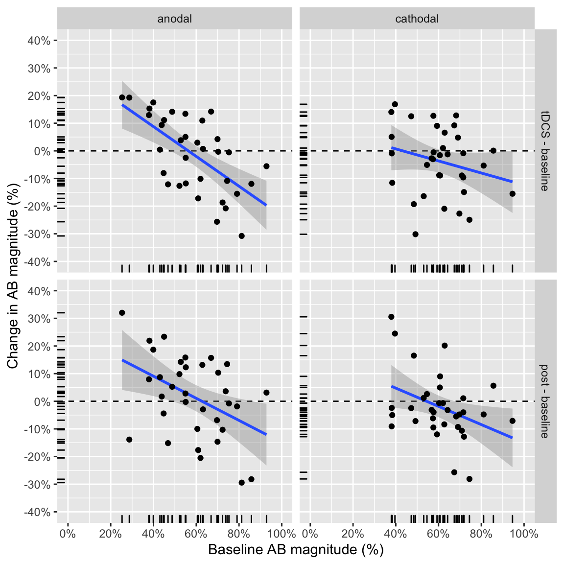
Study 1: change from baseline as a function of baseline performance
Study 2
plot_change_from_baseline(ABmagChange_study2)## `geom_smooth()` using formula 'y ~ x'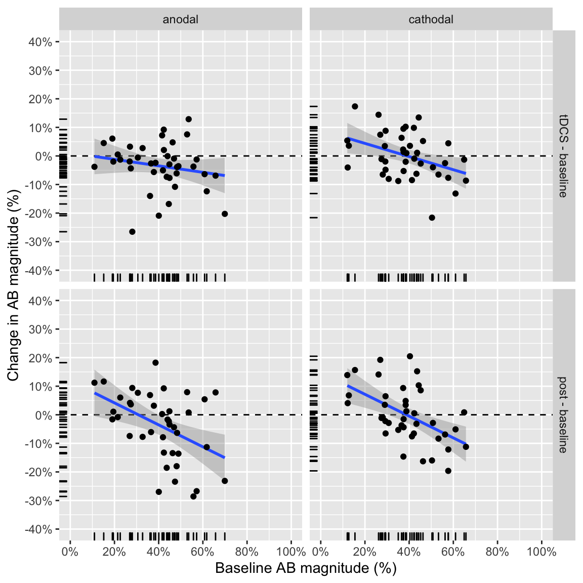
Study 2: change from baseline as a function of baseline performance
Statistics
Partial correlations
pcorr_change_baseline <- function(df) {
  df %>%
    ungroup() %>%
    mutate(session.order = as.numeric(session.order)) %>% # dummy code
    nest_legacy(baseline, change.score, .key = 'value_col') %>% # combine the two performance columns into a list
    # make 2 separate list-columns: AB.magnitude and T1. short
    spread(key = measure, value = value_col) %>% # each contains two vectors: baseline performance and change score
    unnest_legacy(AB.magnitude, T1.short, .sep = '_') %>% # make all 2x2 combinations into 4 columns
    select(-T1.short_baseline) %>% # drop the baseline value for T1.short: not used in partial correlation
    group_by(stimulation,change) %>% # for anodal/cathodal during/after
    # make a data frame out of all 4 columns we need for the partial correlation
    nest_legacy(session.order, AB.magnitude_baseline, AB.magnitude_change.score, T1.short_change.score) %>%
    # partial correlation between baseline and T2|T1 change score, given session order and T1 change score
    mutate(r = map_dbl(data, ~pcor(c("AB.magnitude_baseline","AB.magnitude_change.score",
                                     "session.order", "T1.short_change.score"), var(.)))) %>%
    group_by(stimulation,change) %>%
    mutate(stats = list(as.data.frame(pcor.test(r, 2, n_distinct(df$subject))))) %>% # significance of partial correlations
    unnest_legacy(stats, .drop = TRUE) # combine all into one data frame
}
Partial correlation between:
- baseline AB magnitude
- AB magnitude change from baseline (tDCS - baseline; post - baseline)
Given (adjusing for):
- session order
- change from baseline in T1 accuracy at lag 2
Study 1
kable(pcorr_change_baseline(ABmagChange_study1),
digits = 3, caption = "Study 1: partial correlation change from baseline")| stimulation | change | r | tval | df | pvalue |
|---|---|---|---|---|---|
| anodal | tDCS - baseline | -0.676 | -5.031 | 30 | 0.000 |
| anodal | post - baseline | -0.427 | -2.588 | 30 | 0.015 |
| cathodal | tDCS - baseline | -0.230 | -1.295 | 30 | 0.205 |
| cathodal | post - baseline | -0.381 | -2.258 | 30 | 0.031 |
In study 1, all correlations except for cathodal, tDCS - baseline are significant (without correcting for multiple comparisons). The correlation for anodal, tDCS - baseline is the strongest.
Study 2
kable(pcorr_change_baseline(ABmagChange_study2),
digits = 3, caption = "Study 2: partial correlation change from baseline")| stimulation | change | r | tval | df | pvalue |
|---|---|---|---|---|---|
| anodal | tDCS - baseline | -0.149 | -0.906 | 36 | 0.371 |
| anodal | post - baseline | -0.425 | -2.818 | 36 | 0.008 |
| cathodal | tDCS - baseline | -0.303 | -1.906 | 36 | 0.065 |
| cathodal | post - baseline | -0.443 | -2.969 | 36 | 0.005 |
In study 2, only two correlations are significant: both post - baseline. So the anodal, tDCS - baseline correlation that was the focus of study 1 is not significant here.
Variance tests
There are two problems with assessing the correlation between baseline and change from baseline (retest - baseline, e.g. tDCS - baseline)2.
- Mathematical coupling. The
baselineterm shows up in both variables, introducing a spurious covariance. This may result in a correlation (negative, becausebaselineis subtracted) of up to r = -0.71 (Tu and Gilthorpe, 2007)3, even whenbaselineandretestare randomly sampled from the same distribution. - Regression to the mean. Purely due to measurement error, extreme scores will tend to be less extreme upon another measurement, which also introduces a spurious relation between the two variables.
One solution to regression to the mean is to compare the variances in the baseline and retest. Regression to the mean is a random process, so the variances are expected to be the same. However, if there is truly a relation between baseline and retest - baseline, the variance in the retest should be less than in the baseline: if high-performers become worse, and low-performers become better, so the scores in the retest should be closer together.
Maloney and Rastogi (1970)4 (equation in Tu & Gilthorpe (2007)) and Myrtek and Foerster (1986)5 (equation in Jin (1992)6) propose t-statistics for such tests (which are identical). Further (somewhat counterintuitively), Tu & Gilthorpe (2007) show that testing the variance between baseline and retest is equivalent to testing the significance of the correlation between baseline - retest and baseline + retest (as in Maloney & Rastogi (1970)). Because the sign is now opposite in both variables, the covariance is no longer biased towards either. This illustrates how variance tests also adress mathematical coupling.
var_test <- function(df) {
df %>%
  ungroup() %>%
  select(-T1.short, -session.order) %>% # drop columns we don't need
  spread(block, AB.magnitude) %>% # create 3 columns of scores, one for each block
  gather(condition, retest, tDCS, post) %>% # gather the tdcs and post blocks into one "retest score" column
  unite(comparison, stimulation, condition) %>% # create all 2x2 combinations for the correlations
  group_by(comparison) %>% # for each of these
  nest_legacy() %>% # make a data frame out of the test and retest columns
  mutate(stats = map(data, ~as.data.frame(corr_change_baseline(.$pre, .$retest)))) %>% # apply the variance test
  unnest_legacy(stats, .drop = TRUE) # unpack list into data frame, drop the data
}
Variance tests between:
- baseline AB magnitude (
preblock) - retest AB magnitude (
tDCSorpostblock)
Study 1
kable(var_test(ABmag_study1), digits = 3, caption = "Study 1: test of variance in baseline vs. retest")| comparison | r | df | t | p |
|---|---|---|---|---|
| anodal_tDCS | 0.270 | 32 | 1.584 | 0.123 |
| cathodal_tDCS | -0.198 | 32 | -1.141 | 0.262 |
| anodal_post | -0.018 | 32 | -0.103 | 0.919 |
| cathodal_post | -0.062 | 32 | -0.350 | 0.729 |
Even though three out of four conditions showed a significant negative partial correlation, none of the conditions pass the variance test, suggesting no relation between baseline and change due to tDCS.
Study 2
kable(var_test(ABmag_study2), digits = 3, caption = "Study 2: test of variance in baseline vs. retest")| comparison | r | df | t | p |
|---|---|---|---|---|
| anodal_tDCS | -0.106 | 38 | -0.655 | 0.516 |
| cathodal_tDCS | 0.108 | 38 | 0.671 | 0.507 |
| anodal_post | 0.029 | 38 | 0.177 | 0.860 |
| cathodal_post | 0.183 | 38 | 1.150 | 0.257 |
In study 2 also all variance tests are not significant, again suggesting the two significant partial correlations are spurious.
London, R. E., & Slagter, H. A. (2021). No Effect of Transcranial Direct Current Stimulation over Left Dorsolateral Prefrontal Cortex on Temporal Attention. Journal of Cognitive Neuroscience, 33(4), 756–768. doi: 10.1162/jocn_a_01679↩︎
Taken from this page, which has more extensive introduction to the issue.↩︎
Tu, Y. K., & Gilthorpe, M. S. (2007). Revisiting the relation between change and initial value: a review and evaluation. Statistics in medicine, 26(2), 443-457. doi: 10.1002/sim.2538↩︎
Maloney, C. J., & Rastogi, S. C. (1970). Significance test for Grubbs’s estimators. Biometrics, 26, 671-676.↩︎
Myrtek, M., & Foerster, F. (1986). The law of initial value: A rare exception. Biological Psychology, 22, 227-239.↩︎
Jin, P. (1992). Toward a reconceptualization of the law of initial value. Psychological Bulletin, 111, 176-184. doi: 10.1037/0033-2909.111.1.176↩︎