Setup environment
# Load packages
library(tidyverse)  # importing, transforming, and visualizing data frames
## ── Attaching packages ─────────────────────────────────────── tidyverse 1.3.0 ──## ✓ ggplot2 3.3.3 ✓ purrr 0.3.4
## ✓ tibble 3.0.6 ✓ dplyr 1.0.4
## ✓ tidyr 1.1.2 ✓ stringr 1.4.0
## ✓ readr 1.4.0 ✓ forcats 0.5.1## ── Conflicts ────────────────────────────────────────── tidyverse_conflicts() ──
## x dplyr::filter() masks stats::filter()
## x dplyr::lag() masks stats::lag()library(here) # (relative) file paths## here() starts at /Users/leonreteig/AB-tDCSlibrary(knitr) # R notebook output
library(broom) # transform model outputs into data frames
library(knitrhooks) # printing in rmarkdown outputs
output_max_height()
# Source functions
source(here("src", "func", "behavioral_analysis.R")) # loading data and calculating measures
knitr::read_chunk(here("src", "func", "behavioral_analysis.R")) # display code from file in this
load_data_path <- here("src","func","load_data.Rmd") # for rerunning and displayingnotebookprint(sessionInfo())## R version 3.6.2 (2019-12-12) ## Platform: x86_64-apple-darwin15.6.0 (64-bit) ## Running under: macOS 10.16 ## ## Matrix products: default ## BLAS: /Library/Frameworks/R.framework/Versions/3.6/Resources/lib/libRblas.0.dylib ## LAPACK: /Library/Frameworks/R.framework/Versions/3.6/Resources/lib/libRlapack.dylib ## ## locale: ## [1] en_US.UTF-8/en_US.UTF-8/en_US.UTF-8/C/en_US.UTF-8/en_US.UTF-8 ## ## attached base packages: ## [1] stats graphics grDevices datasets utils methods base ## ## other attached packages: ## [1] knitrhooks_0.0.4 broom_0.7.4.9000 knitr_1.31 here_1.0.1 ## [5] forcats_0.5.1 stringr_1.4.0 dplyr_1.0.4 purrr_0.3.4 ## [9] readr_1.4.0 tidyr_1.1.2 tibble_3.0.6 ggplot2_3.3.3 ## [13] tidyverse_1.3.0 ## ## loaded via a namespace (and not attached): ## [1] tidyselect_1.1.0 xfun_0.21 haven_2.3.1 colorspace_2.0-0 ## [5] vctrs_0.3.6 generics_0.1.0 htmltools_0.5.1.1 yaml_2.2.1 ## [9] rlang_0.4.10 jquerylib_0.1.4 pillar_1.4.7 glue_1.4.2 ## [13] withr_2.4.1 DBI_1.1.1 dbplyr_2.1.0 modelr_0.1.8 ## [17] readxl_1.3.1 lifecycle_1.0.0 munsell_0.5.0 gtable_0.3.0 ## [21] cellranger_1.1.0 rvest_0.3.6 evaluate_0.14 rmdformats_1.0.2 ## [25] Rcpp_1.0.6 renv_0.12.5-72 scales_1.1.1 backports_1.2.1 ## [29] jsonlite_1.7.2 fs_1.5.0 hms_1.0.0 digest_0.6.27 ## [33] stringi_1.5.3 bookdown_0.21 rprojroot_2.0.2 grid_3.6.2 ## [37] cli_2.3.0 tools_3.6.2 magrittr_2.0.1 crayon_1.4.1 ## [41] pkgconfig_2.0.3 ellipsis_0.3.1 xml2_1.3.2 reprex_1.0.0 ## [45] lubridate_1.7.9.2 assertthat_0.2.1 rmarkdown_2.11 httr_1.4.2 ## [49] rstudioapi_0.13 R6_2.5.0 compiler_3.6.2
Load task data
Study 2
The following participants are excluded from further analysis at this point, because of incomplete data:
S03,S14,S29,S38,S43,S46: their T1 performance in session 1 was less than 63% correct, so they were not invited back. This cutoff was determined based on a separate pilot study with 10 participants. It is two standard deviations below the mean of that sample.S25has no data for session 2, as they stopped responding to requests for scheduling the sessionS31was excluded as a precaution after session 1, as they developed a severe headache and we could not rule out the possibility this was related to the tDCS
dataDir_study2 <- here("data") # root folder with AB task data
subs_incomplete <- c("S03", "S14", "S25", "S29", "S31", "S38", "S43", "S46") # don't try to load data from these participants
df_study2 <- load_data_study2(dataDir_study2, subs_incomplete) %>%
  filter(complete.cases(.)) %>% # discard rows with data from incomplete subjects
   # recode first.session ("anodal" or "cathodal") to session.order ("anodal first", "cathodal first")
  mutate(first.session = parse_factor(paste(first.session, "first"),
                                      levels = c("anodal first", "cathodal first"))) %>%
  rename(session.order = first.session)
n_study2 <- n_distinct(df_study2$subject) # number of subjects in study 2kable(head(df_study2,13), digits = 1, caption = "Data frame for study 2")| subject | session.order | stimulation | block | lag | trials | T1 | T2 | T2.given.T1 |
|---|---|---|---|---|---|---|---|---|
| S01 | anodal first | anodal | pre | 3 | 118 | 0.8 | 0.4 | 0.4 |
| S01 | anodal first | anodal | pre | 8 | 60 | 0.8 | 0.8 | 0.8 |
| S01 | anodal first | anodal | tDCS | 3 | 126 | 0.8 | 0.3 | 0.3 |
| S01 | anodal first | anodal | tDCS | 8 | 65 | 0.8 | 0.7 | 0.7 |
| S01 | anodal first | anodal | post | 3 | 122 | 0.8 | 0.2 | 0.3 |
| S01 | anodal first | anodal | post | 8 | 61 | 0.7 | 0.7 | 0.7 |
| S01 | anodal first | cathodal | pre | 3 | 116 | 0.8 | 0.4 | 0.4 |
| S01 | anodal first | cathodal | pre | 8 | 60 | 0.7 | 0.8 | 0.8 |
| S01 | anodal first | cathodal | tDCS | 3 | 129 | 0.7 | 0.4 | 0.4 |
| S01 | anodal first | cathodal | tDCS | 8 | 64 | 0.7 | 0.8 | 0.9 |
| S01 | anodal first | cathodal | post | 3 | 128 | 0.6 | 0.4 | 0.4 |
| S01 | anodal first | cathodal | post | 8 | 62 | 0.7 | 0.8 | 0.8 |
| S02 | cathodal first | anodal | pre | 3 | 124 | 1.0 | 0.8 | 0.8 |
The data has the following columns:
- subject: Participant ID, e.g.
S01,S12 - session.order: Whether participant received
anodalorcathodaltDCS in the first session (anodal_firstvs.cathodal_first). - stimulation: Whether participant received
anodalorcathodaltDCS - block: Whether data is before (
pre), during (tDCS) or after (post`) tDCS - lag: Whether T2 followed T1 after two distractors (lag
3) or after 7 distractors (lag8) - trials: Number of trials per lag that the participant completed in this block
- T1: Proportion of trials (out of
trials) in which T1 was identified correctly - T2: Proportion of trials (out of
trials) in which T2 was identified correctly - T2.given.T1: Proportion of trials which T2 was identified correctly, out of the trials in which T1 was idenitified correctly (T2|T1).
The number of trials vary from person-to-person, as some completed more trials in a 20-minute block than others (because responses were self-paced):
df_study2 %>%
  group_by(lag) %>%
  summarise_at(vars(trials), funs(mean, min, max, sd)) %>%
  kable(caption = "Descriptive statistics for trial counts per lag", digits = 0)
## Warning: `funs()` was deprecated in dplyr 0.8.0.
## Please use a list of either functions or lambdas:
##
## # Simple named list:
## list(mean = mean, median = median)
##
## # Auto named with `tibble::lst()`:
## tibble::lst(mean, median)
##
## # Using lambdas
## list(~ mean(., trim = .2), ~ median(., na.rm = TRUE))| lag | mean | min | max | sd |
|---|---|---|---|---|
| 3 | 130 | 78 | 163 | 17 |
| 8 | 65 | 39 | 87 | 9 |
Study 1
These data were used for statistical analysis in London & Slagter (2021)1, and were processed by the lead author:
dataPath_study1 <- here("data","AB-tDCS_study1.txt")
data_study1_fromDisk <- read.table(dataPath_study1, header = TRUE, dec = ",")
glimpse(data_study1_fromDisk)
## Rows: 34 ## Columns: 120 ## $ SD_T10.3313, 0.0289, -0.8027, -0.5381, -2.… ## $ MeanBLT1Acc 0.8800, 0.8600, 0.8050, 0.8225, 0.665… ## $ First_Session 1, 2, 1, 1, 2, 1, 2, 1, 2, 2, 1, 2, 1… ## $ fileno pp4, pp6, pp7, pp9, pp10, pp11, pp12,… ## $ AB_HighLow 2, 1, 2, 1, 1, 1, 1, 1, 2, 1, 1, 2, 1… ## $ vb_T1_2_NP 0.925, 0.875, 0.825, 0.625, 0.650, 0.… ## $ vb_T1_4_NP 0.800, 0.825, 0.825, 0.825, 0.675, 0.… ## $ vb_T1_10_NP 0.925, 0.925, 0.800, 0.775, 0.825, 0.… ## $ vb_T1_4_P 0.850, 0.900, 0.825, 0.775, 0.625, 0.… ## $ vb_T1_10_P 0.825, 0.900, 0.775, 0.825, 0.625, 0.… ## $ vb_NB_2_NP 0.1351, 0.3429, 0.3636, 0.3600, 0.346… ## $ vb_NB_4_NP 0.3125, 0.5455, 0.5455, 0.3030, 0.296… ## $ vb_NB_10_NP 0.8378, 0.8108, 0.9688, 0.6129, 0.727… ## $ vb_NB_4_P 0.2941, 0.5278, 0.6061, 0.3226, 0.520… ## $ vb_NB_10_P 0.8485, 0.7778, 0.9032, 0.8182, 0.680… ## $ VB_AB 0.7027, 0.4680, 0.6051, 0.2529, 0.381… ## $ VB_REC 0.5253, 0.2654, 0.4233, 0.3099, 0.431… ## $ VB_PE -0.0184, -0.0177, 0.0606, 0.0196, 0.2… ## $ tb_T1_2_NP 0.775, 0.875, 0.675, 0.725, 0.475, 0.… ## $ tb_T1_4_NP 0.825, 0.825, 0.700, 0.750, 0.675, 0.… ## $ tb_T1_10_NP 0.875, 0.900, 0.700, 0.825, 0.500, 0.… ## $ tb_T1_4_P 0.875, 0.800, 0.700, 0.775, 0.650, 0.… ## $ tb_T1_10_P 0.850, 0.925, 0.800, 0.825, 0.625, 0.… ## $ tb_NB_2_NP 0.1290, 0.5143, 0.2222, 0.0690, 0.315… ## $ tb_NB_4_NP 0.3333, 0.5455, 0.6071, 0.1333, 0.370… ## $ tb_NB_10_NP 0.8286, 0.8611, 0.8571, 0.5152, 0.850… ## $ tb_NB_4_P 0.3143, 0.6250, 0.5357, 0.4839, 0.538… ## $ tb_NB_10_P 0.8529, 0.7568, 0.9375, 0.6667, 0.680… ## $ TB_AB 0.6995, 0.3468, 0.6349, 0.4462, 0.534… ## $ TB_REC 0.4952, 0.3157, 0.2500, 0.3818, 0.479… ## $ TB_PE -0.0190, 0.0795, -0.0714, 0.3505, 0.1… ## $ nb_T1_2_NP 0.850, 0.850, 0.650, 0.725, 0.675, 0.… ## $ nb_T1_4_NP 0.800, 0.850, 0.725, 0.675, 0.575, 0.… ## $ nb_T1_10_NP 0.925, 0.825, 0.750, 0.850, 0.725, 0.… ## $ nb_T1_4_P 0.850, 0.900, 0.675, 0.750, 0.875, 0.… ## $ nb_T1_10_P 0.900, 0.825, 0.750, 0.800, 0.550, 0.… ## $ nb_NB_2_NP 0.0588, 0.4412, 0.4615, 0.1034, 0.296… ## $ nb_NB_4_NP 0.0938, 0.4412, 0.2414, 0.1481, 0.478… ## $ nb_NB_10_NP 0.8649, 0.7576, 0.9667, 0.6765, 0.896… ## $ nb_NB_4_P 0.4118, 0.7222, 0.4815, 0.3667, 0.685… ## $ nb_NB_10_P 0.8333, 0.8485, 0.8333, 0.7188, 0.818… ## $ NB_AB 0.8060, 0.3164, 0.5051, 0.5730, 0.600… ## $ NB_REC 0.7711, 0.3164, 0.7253, 0.5283, 0.418… ## $ NB_PE 0.3180, 0.2810, 0.2401, 0.2185, 0.207… ## $ vd_T1_2_NP 0.925, 0.875, 0.800, 0.850, 0.575, 0.… ## $ vd_T1_4_NP 0.850, 0.825, 0.825, 0.925, 0.700, 0.… ## $ vd_T1_10_NP 0.850, 0.900, 0.825, 0.925, 0.750, 0.… ## $ vd_T1_4_P 0.925, 0.775, 0.825, 0.750, 0.650, 0.… ## $ vd_T1_10_P 0.925, 0.800, 0.725, 0.950, 0.575, 0.… ## $ vd_NB_2_NP 0.0541, 0.2857, 0.3125, 0.1765, 0.173… ## $ vd_NB_4_NP 0.2941, 0.4848, 0.4545, 0.2432, 0.428… ## $ vd_NB_10_NP 1.0000, 0.6667, 0.9394, 0.7838, 0.766… ## $ vd_NB_4_P 0.5135, 0.6774, 0.4848, 0.5000, 0.500… ## $ vd_NB_10_P 0.8919, 0.8125, 0.9310, 0.8421, 0.608… ## $ VD_AB 0.9459, 0.3810, 0.6269, 0.6073, 0.592… ## $ VD_REC 0.7059, 0.1818, 0.4848, 0.5405, 0.338… ## $ VD_PE 0.2194, 0.1926, 0.0303, 0.2568, 0.071… ## $ td_T1_2_NP 0.950, 0.775, 0.625, 0.775, 0.525, 0.… ## $ td_T1_4_NP 0.975, 0.800, 0.800, 0.750, 0.625, 0.… ## $ td_T1_10_NP 0.975, 0.900, 0.800, 0.850, 0.575, 0.… ## $ td_T1_4_P 0.875, 0.800, 0.800, 0.800, 0.600, 0.… ## $ td_T1_10_P 0.875, 0.800, 0.850, 0.700, 0.525, 0.… ## $ td_NB_2_NP 0.1579, 0.3226, 0.5200, 0.1290, 0.142… ## $ td_NB_4_NP 0.4615, 0.4375, 0.3750, 0.2333, 0.320… ## $ td_NB_10_NP 0.9487, 0.6944, 0.9375, 0.6471, 0.826… ## $ td_NB_4_P 0.4571, 0.3750, 0.5625, 0.4063, 0.583… ## $ td_NB_10_P 0.8857, 0.6875, 0.8529, 0.7143, 0.666… ## $ TD_AB 0.7908, 0.3719, 0.4175, 0.5180, 0.683… ## $ TD_REC 0.4872, 0.2569, 0.5625, 0.4137, 0.506… ## $ TD_PE -0.0044, -0.0625, 0.1875, 0.1729, 0.2… ## $ nd_T1_2_NP 0.700, 0.800, 0.650, 0.775, 0.425, 0.… ## $ nd_T1_4_NP 0.850, 0.850, 0.725, 0.850, 0.650, 0.… ## $ nd_T1_10_NP 0.800, 0.825, 0.800, 0.850, 0.600, 0.… ## $ nd_T1_4_P 0.850, 0.800, 0.775, 0.775, 0.725, 0.… ## $ nd_T1_10_P 0.850, 0.750, 0.800, 0.850, 0.675, 0.… ## $ nd_NB_2_NP 0.0000, 0.2188, 0.2692, 0.0968, 0.235… ## $ nd_NB_4_NP 0.3824, 0.5000, 0.5172, 0.2353, 0.384… ## $ nd_NB_10_NP 0.8750, 0.5758, 0.8125, 0.7941, 0.708… ## $ nd_NB_4_P 0.4118, 0.5000, 0.5806, 0.5484, 0.482… ## $ nd_NB_10_P 0.9118, 0.7667, 0.8438, 0.8235, 0.629… ## $ ND_AB 0.8750, 0.3570, 0.5433, 0.6973, 0.473… ## $ ND_REC 0.4926, 0.0758, 0.2953, 0.5588, 0.323… ## $ ND_PE 0.0294, 0.0000, 0.0634, 0.3131, 0.098… ## $ AnoMinBl_Lag2_NP -0.01, 0.17, -0.14, -0.29, -0.03, 0.0… ## $ AnoMinBl_Lag10_NP -0.01, 0.05, -0.11, -0.10, 0.12, -0.0… ## $ CathoMinBl_Lag2_NP 0.10, 0.04, 0.21, -0.05, -0.03, 0.09,… ## $ CathoMinBl_Lag10_NP -0.05, 0.03, 0.00, -0.14, 0.06, 0.00,… ## $ Tijdens_AnoMinBl_Lag2_NP -0.01, 0.17, -0.14, -0.29, -0.03, 0.0… ## $ Tijdens_AnoMinBl_Lag10_NP -0.01, 0.05, -0.11, -0.10, 0.12, -0.0… ## $ Tijdens_CathoMinBl_Lag2_NP 0.10, 0.04, 0.21, -0.05, -0.03, 0.09,… ## $ Tijdens_CathoMinBl_Lag10_NP -0.05, 0.03, 0.00, -0.14, 0.06, 0.00,… ## $ Tijdens_AnoMinBL_AB 0.00, -0.12, 0.03, 0.19, 0.15, -0.08,… ## $ Tijdens_CathoMinBL_AB -0.16, -0.01, -0.21, -0.09, 0.09, -0.… ## $ Na_AnoMinBL_AB 0.10, -0.15, -0.10, 0.32, 0.22, -0.04… ## $ Na_CathoMinBL_AB -0.07, -0.02, -0.08, 0.09, -0.12, -0.… ## $ Tijdens_AnoMinBL_PE 0.00, 0.10, -0.13, 0.33, -0.06, -0.06… ## $ Tijdens_CathoMinBL_PE -0.22, -0.26, 0.16, -0.08, 0.19, -0.0… ## $ Na_CathoMinBL_PE -0.19, -0.19, 0.03, 0.06, 0.03, 0.31,… ## $ Na_AnoMinBL_PE 0.34, 0.30, 0.18, 0.20, -0.02, 0.06, … ## $ Tijdens_AnoMinBL_REC -0.03, 0.05, -0.17, 0.07, 0.05, 0.07,… ## $ Tijdens_CathoMinBL_REC -0.22, 0.08, 0.08, -0.13, 0.17, -0.03… ## $ Na_CathoMinBL_REC -0.21, -0.11, -0.19, 0.02, -0.01, 0.1… ## $ Na_AnoMinBL_REC 0.25, 0.05, 0.30, 0.22, -0.01, 0.13, … ## $ T1_Lag2_Tijdens_Ano_Min_BL_NP -0.15, 0.00, -0.15, 0.10, -0.18, 0.00… ## $ T1_Lag2_Tijdens_Catho_Min_BL_NP 0.02, -0.10, -0.18, -0.08, -0.05, -0.… ## $ T1_Lag2_Na_Ano_Min_BL_NP -0.08, -0.03, -0.18, 0.10, 0.03, -0.1… ## $ T1_Lag2_Na_Catho_Min_BL_NP -0.23, -0.08, -0.15, -0.08, -0.15, -0… ## $ T1_Lag4_Tijdens_Ano_Min_BL_NP 0.02, 0.00, -0.13, -0.08, 0.00, 0.05,… ## $ T1_Lag4_Tijdens_Catho_Min_BL_NP 0.13, -0.02, -0.02, -0.18, -0.08, 0.0… ## $ T1_Lag4_Na_Catho_Min_BL_NP 0.00, 0.03, -0.10, -0.08, -0.05, 0.13… ## $ T1_Lag4_Na_Ano_Min_BL_NP 0.00, 0.03, -0.10, -0.15, -0.10, 0.02… ## $ Mean_BL_PE 0.10, 0.09, 0.05, 0.14, 0.15, -0.13, … ## $ ZVB_AB 0.72613, -0.71847, 0.12559, -2.04185,… ## $ ZTB_AB 0.97738, -1.74477, 0.47867, -0.97793,… ## $ ZNB_AB 1.24043, -1.72891, -0.58440, -0.17267… ## $ ZVD_AB 2.47191, -1.64491, 0.14714, 0.00446, … ## $ ZTD_AB 1.39518, -1.23661, -0.94993, -0.31845… ## $ ZND_AB 2.00765, -1.59142, -0.29725, 0.77327,… ## $ VB_T1_Acc_ 0.87, 0.89, 0.81, 0.77, 0.68, 0.95, 0… ## $ VD_T1_Acc_ 0.90, 0.84, 0.80, 0.88, 0.65, 0.90, 0…
We’ll use only a subset of columns, with the header structure block/stim_target_lag_prime, where:
- block/stim is either:
vb: “anodal” tDCS, “pre” block (before tDCS)tb: “anodal” tDCS, “tDCS” block (during tDCS)nb: “anodal” tDCS, “post” block (after tDCS)vd: “cathodal” tDCS, “pre” block (before tDCS)td: “cathodal” tDCS, “tDCS” block (during tDCS)nd: “cathodal” tDCS, “post” block (after tDCS)
- target is either:
T1(T1 accuracy): proportion of trials in which T1 was identified correctlyNB(T2|T1 accuracy): proportion of trials in which T2 was identified correctly, given T1 was identified correctly
- lag is either:
2(lag 2), when T2 followed T1 after 1 distractor4(lag 4), when T2 followed T1 after 3 distractors10, (lag 10), when T2 followed T1 after 9 distractors
- prime is either:
P(prime): when the stimulus at lag 2 (in lag 4 or lag 10 trials) had the same identity as T2NP(no prime) when this was not the case. Study 2 had no primes, so we’ll only keep these.
We’ll also keep two more columns: fileno (participant ID) and First_Session (1 meaning participants received anodal tDCS in the first session, 2 meaning participants received cathodal tDCS in the first session).
Reformat
Now we’ll reformat the data to match the data frame for study 2:
format_study2 <- function(df) {
  df %>%
    select(fileno, First_Session, ends_with("_NP"), -contains("Min")) %>% # keep only relevant columns
    gather(key, accuracy, -fileno, -First_Session) %>% # make long form
    # split key column to create separate columns for each factor
    separate(key, c("block", "stimulation", "target", "lag"), c(1,3,5)) %>% # split after 1st, 3rd, and 5th character
    # convert to factors, relabel levels to match those in study 2
    mutate(block = factor(block, levels = c("v", "t", "n"), labels = c("pre", "tDCS", "post")),
           stimulation = factor(stimulation, levels = c("b_", "d_"), labels = c("anodal", "cathodal")),
           lag = factor(lag, levels = c("_2_NP", "_4_NP", "_10_NP"), labels = c(2, 4, 10)),
           First_Session = factor(First_Session, labels = c("anodal first","cathodal first"))) %>%
    spread(target, accuracy) %>% # create separate columns for T2.given.T1 and T1 performance
    rename(T2.given.T1 = NB, session.order = First_Session, subject = fileno)# rename columns to match those in study 2
}
df_study1 <- format_study2(data_study1_fromDisk)
n_study1 <- n_distinct(df_study1$subject) # number of subjects in study 1kable(head(df_study1,19), digits = 1, caption = "Data frame for study 1")| subject | session.order | block | stimulation | lag | T2.given.T1 | T1 |
|---|---|---|---|---|---|---|
| pp10 | cathodal first | pre | anodal | 2 | 0.3 | 0.6 |
| pp10 | cathodal first | pre | anodal | 4 | 0.3 | 0.7 |
| pp10 | cathodal first | pre | anodal | 10 | 0.7 | 0.8 |
| pp10 | cathodal first | pre | cathodal | 2 | 0.2 | 0.6 |
| pp10 | cathodal first | pre | cathodal | 4 | 0.4 | 0.7 |
| pp10 | cathodal first | pre | cathodal | 10 | 0.8 | 0.8 |
| pp10 | cathodal first | tDCS | anodal | 2 | 0.3 | 0.5 |
| pp10 | cathodal first | tDCS | anodal | 4 | 0.4 | 0.7 |
| pp10 | cathodal first | tDCS | anodal | 10 | 0.8 | 0.5 |
| pp10 | cathodal first | tDCS | cathodal | 2 | 0.1 | 0.5 |
| pp10 | cathodal first | tDCS | cathodal | 4 | 0.3 | 0.6 |
| pp10 | cathodal first | tDCS | cathodal | 10 | 0.8 | 0.6 |
| pp10 | cathodal first | post | anodal | 2 | 0.3 | 0.7 |
| pp10 | cathodal first | post | anodal | 4 | 0.5 | 0.6 |
| pp10 | cathodal first | post | anodal | 10 | 0.9 | 0.7 |
| pp10 | cathodal first | post | cathodal | 2 | 0.2 | 0.4 |
| pp10 | cathodal first | post | cathodal | 4 | 0.4 | 0.6 |
| pp10 | cathodal first | post | cathodal | 10 | 0.7 | 0.6 |
| pp11 | anodal first | pre | anodal | 2 | 0.5 | 1.0 |
Questionnaires
Demographics (study 2)
Load and clean (exclude subjects with incomplete data, and S42 (who did not pass the screening, so had no data)):
subject_info <- read_csv2(here("data", "subject_info.csv"), col_names = TRUE, progress = FALSE, col_types = cols(
  first.session = readr::col_factor(c("anodal", "cathodal")),
  gender = readr::col_factor(c("male", "female")),
  age = col_integer())) %>%
  filter(!(subject %in% c(subs_incomplete, "S42"))) %>%
   # recode first.session ("anodal" or "cathodal") to session.order ("anodal first", "cathodal first")
  mutate(first.session = parse_factor(paste(first.session, "first"),
                                      levels = c("anodal first", "cathodal first"))) %>%
  rename(session.order = first.session)
## ℹ Using ',' as decimal and '.' as grouping mark. Use `read_delim()` for more control.kable(head(subject_info,5), caption = "Demographics in study 2")| subject | session.order | gender | age |
|---|---|---|---|
| S01 | anodal first | female | 20 |
| S02 | cathodal first | female | 19 |
| S04 | anodal first | female | 21 |
| S05 | anodal first | female | 18 |
| S06 | cathodal first | female | 20 |
Analyze:
subject_info %>%
 count(gender) %>%
kable(caption = "Gender breakdown in study 2")| gender | n |
|---|---|
| male | 11 |
| female | 29 |
subject_info %>%
  summarise_at(vars(age), funs(mean, min, max, sd), na.rm = TRUE) %>% # apply summary functions to age column
kable(digits = 2, caption = "Age descriptives in study 2")| mean | min | max | sd |
|---|---|---|---|
| 20.94 | 18 | 28 | 2.48 |
subject_info %>%
 count(session.order) %>%
kable(caption = "Session order breakdown in study 2")| session.order | n |
|---|---|
| anodal first | 18 |
| cathodal first | 22 |
tDCS adverse events (study 2)
Data
tDCS_AE <- read_csv2(here("data", "tDCS_AE.csv"), col_names = TRUE, progress = FALSE, col_types = cols(
  session = readr::col_factor(c("first", "second")),
  stimulation = readr::col_factor(c("anodal", "cathodal"))))
## ℹ Using ',' as decimal and '.' as grouping mark. Use `read_delim()` for more control.glimpse(tDCS_AE)## Rows: 98 ## Columns: 20 ## $ subject"S01", "S01", "S02", "S02", "S03", "S03", "S04", "S04"… ## $ session first, second, first, second, first, second, first, se… ## $ stimulation anodal, cathodal, cathodal, anodal, cathodal, anodal, … ## $ itching 1, 1, 0, 0, 0, 2, 1, 2, 1, 1, 1, 1, 2, 1, 0, 0, 0, 1, … ## $ tingling 1, 1, 3, 1, 1, 1, 3, 0, 2, 2, 0, 1, 2, 1, 1, 1, 1, 0, … ## $ burning 2, 0, 3, 0, 0, 0, 1, 0, 2, 2, 0, 0, 1, 0, 1, 1, 0, 0, … ## $ pain 0, 0, 1, 0, 0, 0, 1, 1, 0, 0, 3, 0, 0, 0, 0, 0, 0, 0, … ## $ headache 1, 0, 2, 1, 1, 0, 0, 3, 1, 1, 2, 4, 0, 0, 0, 1, 0, 3, … ## $ fatigue 1, 0, 1, 0, 0, 0, 2, 3, 2, 2, 2, 4, 1, 1, 2, 2, 3, 2, … ## $ dizziness 0, 0, 1, 0, 0, 0, 0, 0, 0, 0, 0, 0, 1, 0, 0, 0, 0, 0, … ## $ nausea 0, 0, 0, 0, 0, 0, 0, 1, 0, 0, 0, 0, 1, 0, 0, 0, 0, 0, … ## $ conf.itching 3, 3, 0, 0, 0, 4, 3, 3, 3, 3, 4, 4, 4, 3, 0, 0, 0, 4, … ## $ conf.tingling 2, 3, 4, 4, 4, 3, 4, 0, 3, 3, 0, 4, 4, 3, 4, 4, 4, 0, … ## $ conf.burning 3, 0, 4, 0, 0, 0, 3, 0, 4, 3, 0, 0, 4, 0, 4, 4, 0, 0, … ## $ conf.pain 0, 0, 3, 0, 0, 0, 3, 3, 0, 0, 4, 0, 0, 0, 0, 0, 0, 0, … ## $ conf.headache 2, 0, 3, 2, 2, 0, 0, 2, 2, 2, 0, 0, 0, 0, 0, 2, 0, 2, … ## $ conf.fatigue 1, 0, 1, 0, 0, 0, 0, 1, 2, 2, 0, 0, 2, 1, 3, 3, 1, 1, … ## $ conf.dizziness 0, 0, 2, 0, 0, 0, 0, 0, 0, 0, 0, 0, 2, 0, 0, 0, 0, 0, … ## $ conf.nausea 0, 0, 0, 0, 0, 0, 0, 2, 0, 0, 0, 0, 2, 0, 0, 0, 0, 0, … ## $ notes NA, NA, NA, NA, NA, NA, NA, NA, NA, NA, "During the st…
Participants were asked to which degree the following sensations were present during stimulation: tingling, itching sensation, burning sensation, pain, headache, fatigue, dizziness and nausea. Each was rated on a scale from 0-4:
- none
- a little
- moderate
- strong
- very strong
They also rated their confidence that the sensations were caused by the stimulation on a scale from 0-4 (columns starting with conf.):
- n/a (meaning they rated the sensation a 0 on the previous scale)
- unlikely
- possibly
- likely
- very likely
Factors:
- subject: subject ID (
S01,S02, etc) - session: Whether data are from the
firstorsecondsession - stimulation: Whether data are from the
anodalorcathodalsession
Let’s see how many data points we have:
tDCS_AE %>%
  count(stimulation) %>%
kable(caption = "number of completed questionnaires per stimulation type")| stimulation | n |
|---|---|
| anodal | 46 |
| cathodal | 43 |
| NA | 9 |
This is more than the number of subjects (and not the same for anodal and cathodal), because there are a few subjects that only did one session.
For further analysis, make the data long form to easily analyse sensations separately:
# Make long form data frame of sensation intensity
intensity <- tDCS_AE %>%
  select(everything(), -contains("conf"), -notes) %>% # drop other columns
  gather(sensation, intensity, itching:nausea) # make long form

# Make long form data frame of sensation confidence
confidence <- tDCS_AE %>%
  select(contains("conf"), subject, session, stimulation) %>%
  gather(sensation, confidence, conf.itching:conf.nausea) %>%
  mutate(sensation = str_replace(sensation, "conf.", "")) # get rid of "conf." prefix so it matches the sensation intensity table
Let’s see which sensations are reported most frequently, along with their mean level of confidence:
full_join(intensity,confidence) %>%
  group_by(sensation) %>%
  summarise(count = sum(intensity > 0, na.rm = TRUE), # count all occurences (rating "0" means no occurence)
            mean = mean(confidence, na.rm = TRUE)) %>%
  arrange(desc(count)) %>% # most frequent at the top
  kable(digits = 1)
## Joining, by = c("subject", "session", "stimulation", "sensation")| sensation | count | mean |
|---|---|---|
| tingling | 73 | 2.9 |
| itching | 53 | 2.0 |
| fatigue | 52 | 0.8 |
| burning | 40 | 1.6 |
| headache | 27 | 0.6 |
| pain | 11 | 0.4 |
| dizziness | 6 | 0.2 |
| nausea | 5 | 0.2 |
Plot all of the data:
full_join(intensity,confidence)  %>%
  gather(measure, rating, intensity, confidence) %>% # gather confidence/intensity to make one plot for each
  mutate(measure = factor(measure, levels = c("intensity", "confidence"))) %>%

   ggplot(aes(x = rating, fill = stimulation)) +
     facet_grid(measure ~ fct_reorder(sensation, rating, .fun = function(x) sum(x > 0, na.rm = TRUE), .desc = TRUE)) +
    geom_bar(position = "stack") +
    stat_bin(binwidth = 1, geom = "text", size = 2.5, aes(label = ..count..), position = position_stack(vjust = 0.5)) +
    scale_fill_manual(values = c("#F25F5C", "#4B93B1")) +
    xlim(0.5,4.5) + # exclude "0" ratings that were not present
    ylim(0,sum(!is.na(tDCS_AE$stimulation))) + # bound plot at max number of ratings
    ylab("number of sessions") +
    labs(title = "tDCS adverse events", subtitle = "sensations arranged in descending order of frequency")
## Joining, by = c("subject", "session", "stimulation", "sensation")## Warning: Removed 1037 rows containing non-finite values (stat_count).## Warning: Removed 1037 rows containing non-finite values (stat_bin).## Warning: position_stack requires non-overlapping x intervals## Warning: Removed 1 rows containing missing values (geom_bar).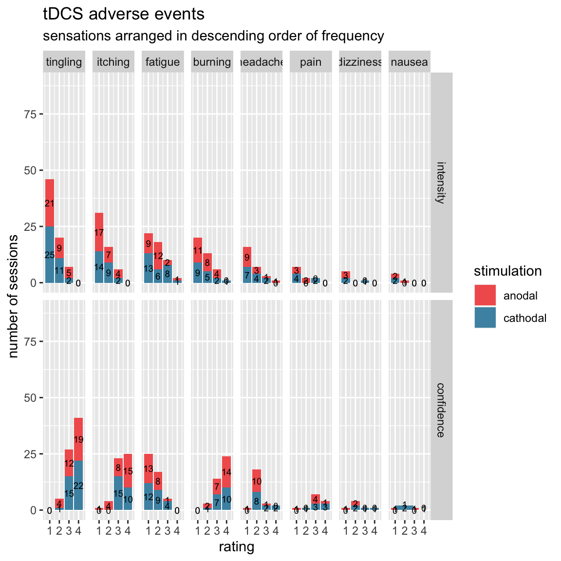
The physical and local sensations (tingling, itching, burning) are most frequent, but these are fairly common and innocuous. Fatigue is also frequent, but there the confidence ratings are highly skewed: participants don’t seem to attribute it to the tDCS. This makes sense as they’ve just done a task for an hour. Headache is still fairly frequent, and has confidence ratings in the middle, which makes sense as headaches often feel “diffuse”. Pain, dizziness and nausea are very rare, and generally low in intensity.
Statistics
Paired Wilcoxon tests for each sensation:
intensity %>%
  filter(!(subject %in% c(subs_incomplete, "S42"))) %>% # set of subjects for which task data are analyzed
  group_by(sensation) %>%
  nest() %>%
  mutate(stats = map(data, ~tidy(wilcox.test(intensity ~ stimulation, paired = TRUE, data = .)))) %>%
  unnest(stats, .drop = TRUE) %>%
  kable(digits = 3, caption = "Paired tests of anodal vs. cathodal for each sensation intensity")
## Warning: The `.drop` argument of `unnest()` is deprecated as of tidyr 1.0.0.
## All list-columns are now preserved.## Warning in wilcox.test.default(x = c(2, 0, 1, 2, 0, 1, 1, 0, 0, 2, 1, 0, :
## cannot compute exact p-value with ties## Warning in wilcox.test.default(x = c(2, 0, 1, 2, 0, 1, 1, 0, 0, 2, 1, 0, :
## cannot compute exact p-value with zeroes## Warning in wilcox.test.default(x = c(0, 0, 0, 0, 0, 1, 0, 0, 0, 0, 0, 0, :
## cannot compute exact p-value with ties## Warning in wilcox.test.default(x = c(0, 0, 0, 0, 0, 1, 0, 0, 0, 0, 0, 0, :
## cannot compute exact p-value with zeroes## Warning in wilcox.test.default(x = c(1, 0, 2, 2, 4, 1, 2, 2, 0, 2, 3, 1, :
## cannot compute exact p-value with ties## Warning in wilcox.test.default(x = c(1, 0, 2, 2, 4, 1, 2, 2, 0, 2, 3, 1, :
## cannot compute exact p-value with zeroes## Warning in wilcox.test.default(x = c(1, 1, 0, 1, 4, 0, 0, 3, 0, 2, 0, 2, :
## cannot compute exact p-value with ties## Warning in wilcox.test.default(x = c(1, 1, 0, 1, 4, 0, 0, 3, 0, 2, 0, 2, :
## cannot compute exact p-value with zeroes## Warning in wilcox.test.default(x = c(1, 0, 1, 1, 1, 2, 0, 1, 1, 1, 3, 0, :
## cannot compute exact p-value with ties## Warning in wilcox.test.default(x = c(1, 0, 1, 1, 1, 2, 0, 1, 1, 1, 3, 0, :
## cannot compute exact p-value with zeroes## Warning in wilcox.test.default(x = c(0, 0, 0, 0, 0, 1, 0, 0, 0, 0, 0, 0, :
## cannot compute exact p-value with ties## Warning in wilcox.test.default(x = c(0, 0, 0, 0, 0, 1, 0, 0, 0, 0, 0, 0, :
## cannot compute exact p-value with zeroes## Warning in wilcox.test.default(x = c(0, 0, 1, 0, 0, 0, 0, 0, 0, 1, 0, 0, :
## cannot compute exact p-value with ties## Warning in wilcox.test.default(x = c(0, 0, 1, 0, 0, 0, 0, 0, 0, 1, 0, 0, :
## cannot compute exact p-value with zeroes## Warning in wilcox.test.default(x = c(1, 1, 3, 2, 1, 2, 1, 0, 1, 2, 0, 0, :
## cannot compute exact p-value with ties## Warning in wilcox.test.default(x = c(1, 1, 3, 2, 1, 2, 1, 0, 1, 2, 0, 0, :
## cannot compute exact p-value with zeroes| sensation | data | statistic | p.value | method | alternative |
|---|---|---|---|---|---|
| itching | S01, S01, S02, S02, S04, S04, S05, S05, S06, S06, S07, S07, S08, S08, S09, S09, S10, S10, S11, S11, S12, S12, S13, S13, S15, S15, S16, S16, S17, S17, S18, S18, S19, S19, S20, S20, S21, S21, S22, S22, S23, S23, S24, S24, S26, S26, S27, S27, S28, S28, S30, S30, S32, S32, S33, S33, S34, S34, S35, S35, S36, S36, S37, S37, S39, S39, S40, S40, S41, S41, S44, S44, S45, S45, S47, S47, S48, S48, S49, S49, 1 , 2 , 1 , 2 , 1 , 2 , 1 , 2 , 1 , 2 , 1 , 2 , 1 , 2 , 1 , 2 , 1 , 2 , 1 , 2 , 1 , 2 , 1 , 2 , 1 , 2 , 1 , 2 , 1 , 2 , 1 , 2 , 1 , 2 , 1 , 2 , 1 , 2 , 1 , 2 , 1 , 2 , 1 , 2 , 1 , 2 , 1 , 2 , 1 , 2 , 1 , 2 , 1 , 2 , 1 , 2 , 1 , 2 , 1 , 2 , 1 , 2 , 1 , 2 , 1 , 2 , 1 , 2 , 1 , 2 , 1 , 2 , 1 , 2 , 1 , 2 , 1 , 2 , 1 , 2 , 1 , 2 , 2 , 1 , 1 , 2 , 1 , 2 , 2 , 1 , 1 , 2 , 1 , 2 , 2 , 1 , 2 , 1 , 1 , 2 , 2 , 1 , 2 , 1 , 1 , 2 , 2 , 1 , 1 , 2 , 2 , 1 , 2 , 1 , 1 , 2 , 2 , 1 , 1 , 2 , 1 , 2 , 2 , 1 , 1 , 2 , 2 , 1 , 2 , 1 , 2 , 1 , 2 , 1 , 1 , 2 , 2 , 1 , 1 , 2 , 2 , 1 , 1 , 2 , 2 , 1 , 1 , 2 , 2 , 1 , 1 , 2 , 2 , 1 , 2 , 1 , 1 , 2 , 2 , 1 , 1 , 1 , 0 , 0 , 1 , 2 , 1 , 1 , 1 , 1 , 2 , 1 , 0 , 0 , 0 , 1 , 1 , 1 , 1 , 0 , 0 , 3 , 1 , 0 , 0 , 2 , 0 , 0 , 1 , 1 , 2 , 3 , 1 , 0 , 0 , 1 , 0 , 0 , 2 , 0 , 0 , 0 , 1 , 0 , 1 , 2 , 0 , 0 , 2 , 0 , 2 , 2 , 3 , 3 , 0 , 0 , 0 , 0 , 0 , 0 , 1 , 2 , 0 , 1 , 2 , 2 , 0 , 0 , 1 , 1 , 2 , 0 , 2 , 1 , 0 , 0 , 1 , 0 , 1 , 1 | 97.0 | 0.949 | Wilcoxon signed rank test with continuity correction | two.sided |
| tingling | S01, S01, S02, S02, S04, S04, S05, S05, S06, S06, S07, S07, S08, S08, S09, S09, S10, S10, S11, S11, S12, S12, S13, S13, S15, S15, S16, S16, S17, S17, S18, S18, S19, S19, S20, S20, S21, S21, S22, S22, S23, S23, S24, S24, S26, S26, S27, S27, S28, S28, S30, S30, S32, S32, S33, S33, S34, S34, S35, S35, S36, S36, S37, S37, S39, S39, S40, S40, S41, S41, S44, S44, S45, S45, S47, S47, S48, S48, S49, S49, 1 , 2 , 1 , 2 , 1 , 2 , 1 , 2 , 1 , 2 , 1 , 2 , 1 , 2 , 1 , 2 , 1 , 2 , 1 , 2 , 1 , 2 , 1 , 2 , 1 , 2 , 1 , 2 , 1 , 2 , 1 , 2 , 1 , 2 , 1 , 2 , 1 , 2 , 1 , 2 , 1 , 2 , 1 , 2 , 1 , 2 , 1 , 2 , 1 , 2 , 1 , 2 , 1 , 2 , 1 , 2 , 1 , 2 , 1 , 2 , 1 , 2 , 1 , 2 , 1 , 2 , 1 , 2 , 1 , 2 , 1 , 2 , 1 , 2 , 1 , 2 , 1 , 2 , 1 , 2 , 1 , 2 , 2 , 1 , 1 , 2 , 1 , 2 , 2 , 1 , 1 , 2 , 1 , 2 , 2 , 1 , 2 , 1 , 1 , 2 , 2 , 1 , 2 , 1 , 1 , 2 , 2 , 1 , 1 , 2 , 2 , 1 , 2 , 1 , 1 , 2 , 2 , 1 , 1 , 2 , 1 , 2 , 2 , 1 , 1 , 2 , 2 , 1 , 2 , 1 , 2 , 1 , 2 , 1 , 1 , 2 , 2 , 1 , 1 , 2 , 2 , 1 , 1 , 2 , 2 , 1 , 1 , 2 , 2 , 1 , 1 , 2 , 2 , 1 , 2 , 1 , 1 , 2 , 2 , 1 , 1 , 1 , 3 , 1 , 3 , 0 , 2 , 2 , 0 , 1 , 2 , 1 , 1 , 1 , 1 , 0 , 1 , 1 , 2 , 0 , 0 , 0 , 2 , 0 , 0 , 2 , 1 , 2 , 1 , 1 , 2 , 3 , 1 , 1 , 0 , 1 , 1 , 1 , 2 , 1 , 2 , 2 , 2 , 1 , 1 , 2 , 1 , 1 , 1 , 0 , 1 , 2 , 3 , 3 , 2 , 2 , 1 , 0 , 1 , 1 , 1 , 1 , 2 , 1 , 1 , 1 , 3 , 1 , 2 , 1 , 0 , 0 , 1 , 1 , 1 , 0 , 1 , 1 , 1 , 1 | 113.0 | 0.942 | Wilcoxon signed rank test with continuity correction | two.sided |
| burning | S01, S01, S02, S02, S04, S04, S05, S05, S06, S06, S07, S07, S08, S08, S09, S09, S10, S10, S11, S11, S12, S12, S13, S13, S15, S15, S16, S16, S17, S17, S18, S18, S19, S19, S20, S20, S21, S21, S22, S22, S23, S23, S24, S24, S26, S26, S27, S27, S28, S28, S30, S30, S32, S32, S33, S33, S34, S34, S35, S35, S36, S36, S37, S37, S39, S39, S40, S40, S41, S41, S44, S44, S45, S45, S47, S47, S48, S48, S49, S49, 1 , 2 , 1 , 2 , 1 , 2 , 1 , 2 , 1 , 2 , 1 , 2 , 1 , 2 , 1 , 2 , 1 , 2 , 1 , 2 , 1 , 2 , 1 , 2 , 1 , 2 , 1 , 2 , 1 , 2 , 1 , 2 , 1 , 2 , 1 , 2 , 1 , 2 , 1 , 2 , 1 , 2 , 1 , 2 , 1 , 2 , 1 , 2 , 1 , 2 , 1 , 2 , 1 , 2 , 1 , 2 , 1 , 2 , 1 , 2 , 1 , 2 , 1 , 2 , 1 , 2 , 1 , 2 , 1 , 2 , 1 , 2 , 1 , 2 , 1 , 2 , 1 , 2 , 1 , 2 , 1 , 2 , 2 , 1 , 1 , 2 , 1 , 2 , 2 , 1 , 1 , 2 , 1 , 2 , 2 , 1 , 2 , 1 , 1 , 2 , 2 , 1 , 2 , 1 , 1 , 2 , 2 , 1 , 1 , 2 , 2 , 1 , 2 , 1 , 1 , 2 , 2 , 1 , 1 , 2 , 1 , 2 , 2 , 1 , 1 , 2 , 2 , 1 , 2 , 1 , 2 , 1 , 2 , 1 , 1 , 2 , 2 , 1 , 1 , 2 , 2 , 1 , 1 , 2 , 2 , 1 , 1 , 2 , 2 , 1 , 1 , 2 , 2 , 1 , 2 , 1 , 1 , 2 , 2 , 1 , 2 , 0 , 3 , 0 , 1 , 0 , 2 , 2 , 0 , 0 , 1 , 0 , 1 , 1 , 0 , 0 , 0 , 0 , 2 , 0 , 4 , 1 , 2 , 0 , 0 , 0 , 0 , 1 , 0 , 0 , 0 , 3 , 1 , 0 , 0 , 0 , 0 , 0 , 1 , 1 , 0 , 0 , 0 , 0 , 3 , 2 , 2 , 0 , 1 , 0 , 1 , 0 , 1 , 2 , 0 , 0 , 0 , 0 , 1 , 0 , 1 , 1 , 2 , 0 , 0 , 0 , 3 , 2 , 0 , 0 , 0 , 0 , 0 , 1 , 0 , 0 , 1 , 0 , 1 , 0 | 131.0 | 0.591 | Wilcoxon signed rank test with continuity correction | two.sided |
| pain | S01, S01, S02, S02, S04, S04, S05, S05, S06, S06, S07, S07, S08, S08, S09, S09, S10, S10, S11, S11, S12, S12, S13, S13, S15, S15, S16, S16, S17, S17, S18, S18, S19, S19, S20, S20, S21, S21, S22, S22, S23, S23, S24, S24, S26, S26, S27, S27, S28, S28, S30, S30, S32, S32, S33, S33, S34, S34, S35, S35, S36, S36, S37, S37, S39, S39, S40, S40, S41, S41, S44, S44, S45, S45, S47, S47, S48, S48, S49, S49, 1 , 2 , 1 , 2 , 1 , 2 , 1 , 2 , 1 , 2 , 1 , 2 , 1 , 2 , 1 , 2 , 1 , 2 , 1 , 2 , 1 , 2 , 1 , 2 , 1 , 2 , 1 , 2 , 1 , 2 , 1 , 2 , 1 , 2 , 1 , 2 , 1 , 2 , 1 , 2 , 1 , 2 , 1 , 2 , 1 , 2 , 1 , 2 , 1 , 2 , 1 , 2 , 1 , 2 , 1 , 2 , 1 , 2 , 1 , 2 , 1 , 2 , 1 , 2 , 1 , 2 , 1 , 2 , 1 , 2 , 1 , 2 , 1 , 2 , 1 , 2 , 1 , 2 , 1 , 2 , 1 , 2 , 2 , 1 , 1 , 2 , 1 , 2 , 2 , 1 , 1 , 2 , 1 , 2 , 2 , 1 , 2 , 1 , 1 , 2 , 2 , 1 , 2 , 1 , 1 , 2 , 2 , 1 , 1 , 2 , 2 , 1 , 2 , 1 , 1 , 2 , 2 , 1 , 1 , 2 , 1 , 2 , 2 , 1 , 1 , 2 , 2 , 1 , 2 , 1 , 2 , 1 , 2 , 1 , 1 , 2 , 2 , 1 , 1 , 2 , 2 , 1 , 1 , 2 , 2 , 1 , 1 , 2 , 2 , 1 , 1 , 2 , 2 , 1 , 2 , 1 , 1 , 2 , 2 , 1 , 0 , 0 , 1 , 0 , 1 , 1 , 0 , 0 , 3 , 0 , 0 , 0 , 0 , 0 , 0 , 0 , 0 , 0 , 1 , 0 , 0 , 0 , 1 , 0 , 0 , 0 , 0 , 0 , 0 , 0 , 1 , 1 , 0 , 0 , 0 , 0 , 0 , 0 , 0 , 0 , 0 , 0 , 0 , 0 , 0 , 0 , 0 , 0 , 0 , 0 , 0 , 0 , 0 , 0 , 0 , 0 , 0 , 0 , 0 , 0 , 0 , 0 , 0 , 0 , 0 , 0 , 0 , 3 , 0 , 0 , 2 , 0 , 0 , 0 , 0 , 0 , 0 , 0 , 0 , 0 | 6.0 | 0.395 | Wilcoxon signed rank test with continuity correction | two.sided |
| headache | S01, S01, S02, S02, S04, S04, S05, S05, S06, S06, S07, S07, S08, S08, S09, S09, S10, S10, S11, S11, S12, S12, S13, S13, S15, S15, S16, S16, S17, S17, S18, S18, S19, S19, S20, S20, S21, S21, S22, S22, S23, S23, S24, S24, S26, S26, S27, S27, S28, S28, S30, S30, S32, S32, S33, S33, S34, S34, S35, S35, S36, S36, S37, S37, S39, S39, S40, S40, S41, S41, S44, S44, S45, S45, S47, S47, S48, S48, S49, S49, 1 , 2 , 1 , 2 , 1 , 2 , 1 , 2 , 1 , 2 , 1 , 2 , 1 , 2 , 1 , 2 , 1 , 2 , 1 , 2 , 1 , 2 , 1 , 2 , 1 , 2 , 1 , 2 , 1 , 2 , 1 , 2 , 1 , 2 , 1 , 2 , 1 , 2 , 1 , 2 , 1 , 2 , 1 , 2 , 1 , 2 , 1 , 2 , 1 , 2 , 1 , 2 , 1 , 2 , 1 , 2 , 1 , 2 , 1 , 2 , 1 , 2 , 1 , 2 , 1 , 2 , 1 , 2 , 1 , 2 , 1 , 2 , 1 , 2 , 1 , 2 , 1 , 2 , 1 , 2 , 1 , 2 , 2 , 1 , 1 , 2 , 1 , 2 , 2 , 1 , 1 , 2 , 1 , 2 , 2 , 1 , 2 , 1 , 1 , 2 , 2 , 1 , 2 , 1 , 1 , 2 , 2 , 1 , 1 , 2 , 2 , 1 , 2 , 1 , 1 , 2 , 2 , 1 , 1 , 2 , 1 , 2 , 2 , 1 , 1 , 2 , 2 , 1 , 2 , 1 , 2 , 1 , 2 , 1 , 1 , 2 , 2 , 1 , 1 , 2 , 2 , 1 , 1 , 2 , 2 , 1 , 1 , 2 , 2 , 1 , 1 , 2 , 2 , 1 , 2 , 1 , 1 , 2 , 2 , 1 , 1 , 0 , 2 , 1 , 0 , 3 , 1 , 1 , 2 , 4 , 0 , 0 , 0 , 1 , 0 , 3 , 0 , 0 , 2 , 1 , 1 , 0 , 2 , 2 , 0 , 0 , 0 , 0 , 0 , 0 , 0 , 1 , 1 , 0 , 0 , 0 , 0 , 0 , 0 , 0 , 0 , 0 , 0 , 0 , 0 , 0 , 0 , 0 , 0 , 0 , 0 , 0 , 2 , 0 , 0 , 0 , 0 , 0 , 0 , 0 , 0 , 0 , 0 , 0 , 0 , 0 , 1 , 3 , 0 , 0 , 0 , 0 , 0 , 1 , 0 , 0 , 1 , 0 , 0 , 0 | 49.5 | 0.871 | Wilcoxon signed rank test with continuity correction | two.sided |
| fatigue | S01, S01, S02, S02, S04, S04, S05, S05, S06, S06, S07, S07, S08, S08, S09, S09, S10, S10, S11, S11, S12, S12, S13, S13, S15, S15, S16, S16, S17, S17, S18, S18, S19, S19, S20, S20, S21, S21, S22, S22, S23, S23, S24, S24, S26, S26, S27, S27, S28, S28, S30, S30, S32, S32, S33, S33, S34, S34, S35, S35, S36, S36, S37, S37, S39, S39, S40, S40, S41, S41, S44, S44, S45, S45, S47, S47, S48, S48, S49, S49, 1 , 2 , 1 , 2 , 1 , 2 , 1 , 2 , 1 , 2 , 1 , 2 , 1 , 2 , 1 , 2 , 1 , 2 , 1 , 2 , 1 , 2 , 1 , 2 , 1 , 2 , 1 , 2 , 1 , 2 , 1 , 2 , 1 , 2 , 1 , 2 , 1 , 2 , 1 , 2 , 1 , 2 , 1 , 2 , 1 , 2 , 1 , 2 , 1 , 2 , 1 , 2 , 1 , 2 , 1 , 2 , 1 , 2 , 1 , 2 , 1 , 2 , 1 , 2 , 1 , 2 , 1 , 2 , 1 , 2 , 1 , 2 , 1 , 2 , 1 , 2 , 1 , 2 , 1 , 2 , 1 , 2 , 2 , 1 , 1 , 2 , 1 , 2 , 2 , 1 , 1 , 2 , 1 , 2 , 2 , 1 , 2 , 1 , 1 , 2 , 2 , 1 , 2 , 1 , 1 , 2 , 2 , 1 , 1 , 2 , 2 , 1 , 2 , 1 , 1 , 2 , 2 , 1 , 1 , 2 , 1 , 2 , 2 , 1 , 1 , 2 , 2 , 1 , 2 , 1 , 2 , 1 , 2 , 1 , 1 , 2 , 2 , 1 , 1 , 2 , 2 , 1 , 1 , 2 , 2 , 1 , 1 , 2 , 2 , 1 , 1 , 2 , 2 , 1 , 2 , 1 , 1 , 2 , 2 , 1 , 1 , 0 , 1 , 0 , 2 , 3 , 2 , 2 , 2 , 4 , 1 , 1 , 2 , 2 , 3 , 2 , 0 , 0 , 2 , 0 , 3 , 3 , 1 , 1 , 2 , 2 , 2 , 0 , 0 , 0 , 0 , 1 , 1 , 0 , 2 , 0 , 1 , 0 , 2 , 3 , 1 , 0 , 3 , 2 , 0 , 0 , 1 , 0 , 1 , 0 , 0 , 0 , 1 , 1 , 2 , 2 , 0 , 0 , 0 , 0 , 0 , 0 , 1 , 3 , 1 , 1 , 3 , 3 , 1 , 0 , 0 , 1 , 0 , 0 , 0 , 0 , 2 , 3 , 1 , 0 | 82.5 | 0.232 | Wilcoxon signed rank test with continuity correction | two.sided |
| dizziness | S01, S01, S02, S02, S04, S04, S05, S05, S06, S06, S07, S07, S08, S08, S09, S09, S10, S10, S11, S11, S12, S12, S13, S13, S15, S15, S16, S16, S17, S17, S18, S18, S19, S19, S20, S20, S21, S21, S22, S22, S23, S23, S24, S24, S26, S26, S27, S27, S28, S28, S30, S30, S32, S32, S33, S33, S34, S34, S35, S35, S36, S36, S37, S37, S39, S39, S40, S40, S41, S41, S44, S44, S45, S45, S47, S47, S48, S48, S49, S49, 1 , 2 , 1 , 2 , 1 , 2 , 1 , 2 , 1 , 2 , 1 , 2 , 1 , 2 , 1 , 2 , 1 , 2 , 1 , 2 , 1 , 2 , 1 , 2 , 1 , 2 , 1 , 2 , 1 , 2 , 1 , 2 , 1 , 2 , 1 , 2 , 1 , 2 , 1 , 2 , 1 , 2 , 1 , 2 , 1 , 2 , 1 , 2 , 1 , 2 , 1 , 2 , 1 , 2 , 1 , 2 , 1 , 2 , 1 , 2 , 1 , 2 , 1 , 2 , 1 , 2 , 1 , 2 , 1 , 2 , 1 , 2 , 1 , 2 , 1 , 2 , 1 , 2 , 1 , 2 , 1 , 2 , 2 , 1 , 1 , 2 , 1 , 2 , 2 , 1 , 1 , 2 , 1 , 2 , 2 , 1 , 2 , 1 , 1 , 2 , 2 , 1 , 2 , 1 , 1 , 2 , 2 , 1 , 1 , 2 , 2 , 1 , 2 , 1 , 1 , 2 , 2 , 1 , 1 , 2 , 1 , 2 , 2 , 1 , 1 , 2 , 2 , 1 , 2 , 1 , 2 , 1 , 2 , 1 , 1 , 2 , 2 , 1 , 1 , 2 , 2 , 1 , 1 , 2 , 2 , 1 , 1 , 2 , 2 , 1 , 1 , 2 , 2 , 1 , 2 , 1 , 1 , 2 , 2 , 1 , 0 , 0 , 1 , 0 , 0 , 0 , 0 , 0 , 0 , 0 , 1 , 0 , 0 , 0 , 0 , 0 , 0 , 0 , 0 , 0 , 0 , 0 , 0 , 0 , 0 , 0 , 0 , 0 , 0 , 0 , 0 , 0 , 0 , 0 , 0 , 0 , 0 , 0 , 0 , 0 , 0 , 0 , 0 , 0 , 0 , 0 , 0 , 0 , 0 , 0 , 0 , 0 , 0 , 0 , 1 , 1 , 0 , 0 , 0 , 0 , 0 , 0 , 0 , 0 , 0 , 0 , 0 , 0 , 0 , 0 , 0 , 0 , 0 , 0 , 0 , 0 , 0 , 0 , 0 , 0 | 1.5 | 1.000 | Wilcoxon signed rank test with continuity correction | two.sided |
| nausea | S01, S01, S02, S02, S04, S04, S05, S05, S06, S06, S07, S07, S08, S08, S09, S09, S10, S10, S11, S11, S12, S12, S13, S13, S15, S15, S16, S16, S17, S17, S18, S18, S19, S19, S20, S20, S21, S21, S22, S22, S23, S23, S24, S24, S26, S26, S27, S27, S28, S28, S30, S30, S32, S32, S33, S33, S34, S34, S35, S35, S36, S36, S37, S37, S39, S39, S40, S40, S41, S41, S44, S44, S45, S45, S47, S47, S48, S48, S49, S49, 1 , 2 , 1 , 2 , 1 , 2 , 1 , 2 , 1 , 2 , 1 , 2 , 1 , 2 , 1 , 2 , 1 , 2 , 1 , 2 , 1 , 2 , 1 , 2 , 1 , 2 , 1 , 2 , 1 , 2 , 1 , 2 , 1 , 2 , 1 , 2 , 1 , 2 , 1 , 2 , 1 , 2 , 1 , 2 , 1 , 2 , 1 , 2 , 1 , 2 , 1 , 2 , 1 , 2 , 1 , 2 , 1 , 2 , 1 , 2 , 1 , 2 , 1 , 2 , 1 , 2 , 1 , 2 , 1 , 2 , 1 , 2 , 1 , 2 , 1 , 2 , 1 , 2 , 1 , 2 , 1 , 2 , 2 , 1 , 1 , 2 , 1 , 2 , 2 , 1 , 1 , 2 , 1 , 2 , 2 , 1 , 2 , 1 , 1 , 2 , 2 , 1 , 2 , 1 , 1 , 2 , 2 , 1 , 1 , 2 , 2 , 1 , 2 , 1 , 1 , 2 , 2 , 1 , 1 , 2 , 1 , 2 , 2 , 1 , 1 , 2 , 2 , 1 , 2 , 1 , 2 , 1 , 2 , 1 , 1 , 2 , 2 , 1 , 1 , 2 , 2 , 1 , 1 , 2 , 2 , 1 , 1 , 2 , 2 , 1 , 1 , 2 , 2 , 1 , 2 , 1 , 1 , 2 , 2 , 1 , 0 , 0 , 0 , 0 , 0 , 1 , 0 , 0 , 0 , 0 , 1 , 0 , 0 , 0 , 0 , 0 , 0 , 0 , 0 , 0 , 0 , 0 , 0 , 0 , 0 , 0 , 0 , 0 , 0 , 0 , 0 , 0 , 0 , 0 , 0 , 0 , 0 , 0 , 0 , 0 , 0 , 0 , 0 , 0 , 0 , 0 , 0 , 0 , 0 , 0 , 0 , 0 , 0 , 0 , 0 , 0 , 0 , 0 , 0 , 0 , 0 , 0 , 0 , 0 , 0 , 0 , 0 , 1 , 0 , 0 , 0 , 0 , 0 , 0 , 0 , 0 , 0 , 0 , 0 , 0 | 2.0 | 0.773 | Wilcoxon signed rank test with continuity correction | two.sided |
London, R. E., & Slagter, H. A. (2021). No Effect of Transcranial Direct Current Stimulation over Left Dorsolateral Prefrontal Cortex on Temporal Attention. Journal of Cognitive Neuroscience, 33(4), 756–768. doi: 10.1162/jocn_a_01679↩︎