# Load packages
library(tidyverse)  # importing, transforming, and visualizing data frames
## ── Attaching packages ─────────────────────────────────────── tidyverse 1.3.0 ──## ✓ ggplot2 3.3.3 ✓ purrr 0.3.4
## ✓ tibble 3.0.6 ✓ dplyr 1.0.4
## ✓ tidyr 1.1.2 ✓ stringr 1.4.0
## ✓ readr 1.4.0 ✓ forcats 0.5.1## ── Conflicts ────────────────────────────────────────── tidyverse_conflicts() ──
## x dplyr::filter() masks stats::filter()
## x dplyr::lag() masks stats::lag()library(here) # (relative) file paths## here() starts at /Users/leonreteig/AB-tDCSlibrary(knitr) # R notebook output
library(scales) # Percentage axis labels ##
## Attaching package: 'scales'## The following object is masked from 'package:purrr':
##
## discard## The following object is masked from 'package:readr':
##
## col_factorlibrary(broom) # transform model outputs into data frames
library(ggm) # partial correlations
library(BayesFactor) # Bayesian statistics## Loading required package: coda## Loading required package: Matrix##
## Attaching package: 'Matrix'## The following objects are masked from 'package:tidyr':
##
## expand, pack, unpack## ************
## Welcome to BayesFactor 0.9.12-4.2. If you have questions, please contact Richard Morey (richarddmorey@gmail.com).
##
## Type BFManual() to open the manual.
## ************library(knitrhooks) # printing in rmarkdown outputs
output_max_height()
# Source functions
source(here("src", "func", "behavioral_analysis.R")) # loading data and calculating measures
load_data_path <- here("src","func","load_data.Rmd") # for rerunning and displaying
knitr::read_chunk(here("src", "func", "behavioral_analysis.R")) # display code from file in this notebookprint(sessionInfo())## R version 3.6.2 (2019-12-12) ## Platform: x86_64-apple-darwin15.6.0 (64-bit) ## Running under: macOS 10.16 ## ## Matrix products: default ## BLAS: /Library/Frameworks/R.framework/Versions/3.6/Resources/lib/libRblas.0.dylib ## LAPACK: /Library/Frameworks/R.framework/Versions/3.6/Resources/lib/libRlapack.dylib ## ## locale: ## [1] en_US.UTF-8/en_US.UTF-8/en_US.UTF-8/C/en_US.UTF-8/en_US.UTF-8 ## ## attached base packages: ## [1] stats graphics grDevices datasets utils methods base ## ## other attached packages: ## [1] knitrhooks_0.0.4 BayesFactor_0.9.12-4.2 Matrix_1.3-2 ## [4] coda_0.19-4 ggm_2.5 broom_0.7.4.9000 ## [7] scales_1.1.1 knitr_1.31 here_1.0.1 ## [10] forcats_0.5.1 stringr_1.4.0 dplyr_1.0.4 ## [13] purrr_0.3.4 readr_1.4.0 tidyr_1.1.2 ## [16] tibble_3.0.6 ggplot2_3.3.3 tidyverse_1.3.0 ## ## loaded via a namespace (and not attached): ## [1] Rcpp_1.0.6 lubridate_1.7.9.2 mvtnorm_1.1-1 lattice_0.20-41 ## [5] gtools_3.8.2 assertthat_0.2.1 rprojroot_2.0.2 digest_0.6.27 ## [9] R6_2.5.0 cellranger_1.1.0 backports_1.2.1 MatrixModels_0.5-0 ## [13] reprex_1.0.0 evaluate_0.14 httr_1.4.2 pillar_1.4.7 ## [17] rlang_0.4.10 readxl_1.3.1 rstudioapi_0.13 jquerylib_0.1.4 ## [21] rmarkdown_2.11 igraph_1.2.6 munsell_0.5.0 compiler_3.6.2 ## [25] modelr_0.1.8 xfun_0.21 pkgconfig_2.0.3 htmltools_0.5.1.1 ## [29] tidyselect_1.1.0 bookdown_0.21 crayon_1.4.1 dbplyr_2.1.0 ## [33] withr_2.4.1 grid_3.6.2 jsonlite_1.7.2 gtable_0.3.0 ## [37] lifecycle_1.0.0 DBI_1.1.1 magrittr_2.0.1 rmdformats_1.0.2 ## [41] cli_2.3.0 stringi_1.5.3 pbapply_1.4-3 renv_0.12.5-72 ## [45] fs_1.5.0 xml2_1.3.2 ellipsis_0.3.1 generics_0.1.0 ## [49] vctrs_0.3.6 tools_3.6.2 glue_1.4.2 hms_1.0.0 ## [53] parallel_3.6.2 yaml_2.2.1 colorspace_2.0-0 rvest_0.3.6 ## [57] haven_2.3.1
Load task data
Study 2
The following participants are excluded from further analysis at this point, because of incomplete data:
S03,S14,S29,S38,S43,S46: their T1 performance in session 1 was less than 63% correct, so they were not invited back. This cutoff was determined based on a separate pilot study with 10 participants. It is two standard deviations below the mean of that sample.S25has no data for session 2, as they stopped responding to requests for scheduling the sessionS31was excluded as a precaution after session 1, as they developed a severe headache and we could not rule out the possibility this was related to the tDCS
dataDir_study2 <- here("data") # root folder with AB task data
subs_incomplete <- c("S03", "S14", "S25", "S29", "S31", "S38", "S43", "S46") # don't try to load data from these participants
df_study2 <- load_data_study2(dataDir_study2, subs_incomplete) %>%
  filter(complete.cases(.)) %>% # discard rows with data from incomplete subjects
   # recode first.session ("anodal" or "cathodal") to session.order ("anodal first", "cathodal first")
  mutate(first.session = parse_factor(paste(first.session, "first"),
                                      levels = c("anodal first", "cathodal first"))) %>%
  rename(session.order = first.session)
n_study2 <- n_distinct(df_study2$subject) # number of subjects in study 2kable(head(df_study2,13), digits = 1, caption = "Data frame for study 2")| subject | session.order | stimulation | block | lag | trials | T1 | T2 | T2.given.T1 |
|---|---|---|---|---|---|---|---|---|
| S01 | anodal first | anodal | pre | 3 | 118 | 0.8 | 0.4 | 0.4 |
| S01 | anodal first | anodal | pre | 8 | 60 | 0.8 | 0.8 | 0.8 |
| S01 | anodal first | anodal | tDCS | 3 | 126 | 0.8 | 0.3 | 0.3 |
| S01 | anodal first | anodal | tDCS | 8 | 65 | 0.8 | 0.7 | 0.7 |
| S01 | anodal first | anodal | post | 3 | 122 | 0.8 | 0.2 | 0.3 |
| S01 | anodal first | anodal | post | 8 | 61 | 0.7 | 0.7 | 0.7 |
| S01 | anodal first | cathodal | pre | 3 | 116 | 0.8 | 0.4 | 0.4 |
| S01 | anodal first | cathodal | pre | 8 | 60 | 0.7 | 0.8 | 0.8 |
| S01 | anodal first | cathodal | tDCS | 3 | 129 | 0.7 | 0.4 | 0.4 |
| S01 | anodal first | cathodal | tDCS | 8 | 64 | 0.7 | 0.8 | 0.9 |
| S01 | anodal first | cathodal | post | 3 | 128 | 0.6 | 0.4 | 0.4 |
| S01 | anodal first | cathodal | post | 8 | 62 | 0.7 | 0.8 | 0.8 |
| S02 | cathodal first | anodal | pre | 3 | 124 | 1.0 | 0.8 | 0.8 |
The data has the following columns:
- subject: Participant ID, e.g.
S01,S12 - session.order: Whether participant received
anodalorcathodaltDCS in the first session (anodal_firstvs.cathodal_first). - stimulation: Whether participant received
anodalorcathodaltDCS - block: Whether data is before (
pre), during (tDCS) or after (post`) tDCS - lag: Whether T2 followed T1 after two distractors (lag
3) or after 7 distractors (lag8) - trials: Number of trials per lag that the participant completed in this block
- T1: Proportion of trials (out of
trials) in which T1 was identified correctly - T2: Proportion of trials (out of
trials) in which T2 was identified correctly - T2.given.T1: Proportion of trials which T2 was identified correctly, out of the trials in which T1 was idenitified correctly (T2|T1).
The number of trials vary from person-to-person, as some completed more trials in a 20-minute block than others (because responses were self-paced):
df_study2 %>%
  group_by(lag) %>%
  summarise_at(vars(trials), funs(mean, min, max, sd)) %>%
  kable(caption = "Descriptive statistics for trial counts per lag", digits = 0)
## Warning: `funs()` was deprecated in dplyr 0.8.0.
## Please use a list of either functions or lambdas:
##
## # Simple named list:
## list(mean = mean, median = median)
##
## # Auto named with `tibble::lst()`:
## tibble::lst(mean, median)
##
## # Using lambdas
## list(~ mean(., trim = .2), ~ median(., na.rm = TRUE))| lag | mean | min | max | sd |
|---|---|---|---|---|
| 3 | 130 | 78 | 163 | 17 |
| 8 | 65 | 39 | 87 | 9 |
Study 1
These data were used for statistical analysis in London & Slagter (2021)1, and were processed by the lead author:
dataPath_study1 <- here("data","AB-tDCS_study1.txt")
data_study1_fromDisk <- read.table(dataPath_study1, header = TRUE, dec = ",")
glimpse(data_study1_fromDisk)
## Rows: 34 ## Columns: 120 ## $ SD_T10.3313, 0.0289, -0.8027, -0.5381, -2.… ## $ MeanBLT1Acc 0.8800, 0.8600, 0.8050, 0.8225, 0.665… ## $ First_Session 1, 2, 1, 1, 2, 1, 2, 1, 2, 2, 1, 2, 1… ## $ fileno pp4, pp6, pp7, pp9, pp10, pp11, pp12,… ## $ AB_HighLow 2, 1, 2, 1, 1, 1, 1, 1, 2, 1, 1, 2, 1… ## $ vb_T1_2_NP 0.925, 0.875, 0.825, 0.625, 0.650, 0.… ## $ vb_T1_4_NP 0.800, 0.825, 0.825, 0.825, 0.675, 0.… ## $ vb_T1_10_NP 0.925, 0.925, 0.800, 0.775, 0.825, 0.… ## $ vb_T1_4_P 0.850, 0.900, 0.825, 0.775, 0.625, 0.… ## $ vb_T1_10_P 0.825, 0.900, 0.775, 0.825, 0.625, 0.… ## $ vb_NB_2_NP 0.1351, 0.3429, 0.3636, 0.3600, 0.346… ## $ vb_NB_4_NP 0.3125, 0.5455, 0.5455, 0.3030, 0.296… ## $ vb_NB_10_NP 0.8378, 0.8108, 0.9688, 0.6129, 0.727… ## $ vb_NB_4_P 0.2941, 0.5278, 0.6061, 0.3226, 0.520… ## $ vb_NB_10_P 0.8485, 0.7778, 0.9032, 0.8182, 0.680… ## $ VB_AB 0.7027, 0.4680, 0.6051, 0.2529, 0.381… ## $ VB_REC 0.5253, 0.2654, 0.4233, 0.3099, 0.431… ## $ VB_PE -0.0184, -0.0177, 0.0606, 0.0196, 0.2… ## $ tb_T1_2_NP 0.775, 0.875, 0.675, 0.725, 0.475, 0.… ## $ tb_T1_4_NP 0.825, 0.825, 0.700, 0.750, 0.675, 0.… ## $ tb_T1_10_NP 0.875, 0.900, 0.700, 0.825, 0.500, 0.… ## $ tb_T1_4_P 0.875, 0.800, 0.700, 0.775, 0.650, 0.… ## $ tb_T1_10_P 0.850, 0.925, 0.800, 0.825, 0.625, 0.… ## $ tb_NB_2_NP 0.1290, 0.5143, 0.2222, 0.0690, 0.315… ## $ tb_NB_4_NP 0.3333, 0.5455, 0.6071, 0.1333, 0.370… ## $ tb_NB_10_NP 0.8286, 0.8611, 0.8571, 0.5152, 0.850… ## $ tb_NB_4_P 0.3143, 0.6250, 0.5357, 0.4839, 0.538… ## $ tb_NB_10_P 0.8529, 0.7568, 0.9375, 0.6667, 0.680… ## $ TB_AB 0.6995, 0.3468, 0.6349, 0.4462, 0.534… ## $ TB_REC 0.4952, 0.3157, 0.2500, 0.3818, 0.479… ## $ TB_PE -0.0190, 0.0795, -0.0714, 0.3505, 0.1… ## $ nb_T1_2_NP 0.850, 0.850, 0.650, 0.725, 0.675, 0.… ## $ nb_T1_4_NP 0.800, 0.850, 0.725, 0.675, 0.575, 0.… ## $ nb_T1_10_NP 0.925, 0.825, 0.750, 0.850, 0.725, 0.… ## $ nb_T1_4_P 0.850, 0.900, 0.675, 0.750, 0.875, 0.… ## $ nb_T1_10_P 0.900, 0.825, 0.750, 0.800, 0.550, 0.… ## $ nb_NB_2_NP 0.0588, 0.4412, 0.4615, 0.1034, 0.296… ## $ nb_NB_4_NP 0.0938, 0.4412, 0.2414, 0.1481, 0.478… ## $ nb_NB_10_NP 0.8649, 0.7576, 0.9667, 0.6765, 0.896… ## $ nb_NB_4_P 0.4118, 0.7222, 0.4815, 0.3667, 0.685… ## $ nb_NB_10_P 0.8333, 0.8485, 0.8333, 0.7188, 0.818… ## $ NB_AB 0.8060, 0.3164, 0.5051, 0.5730, 0.600… ## $ NB_REC 0.7711, 0.3164, 0.7253, 0.5283, 0.418… ## $ NB_PE 0.3180, 0.2810, 0.2401, 0.2185, 0.207… ## $ vd_T1_2_NP 0.925, 0.875, 0.800, 0.850, 0.575, 0.… ## $ vd_T1_4_NP 0.850, 0.825, 0.825, 0.925, 0.700, 0.… ## $ vd_T1_10_NP 0.850, 0.900, 0.825, 0.925, 0.750, 0.… ## $ vd_T1_4_P 0.925, 0.775, 0.825, 0.750, 0.650, 0.… ## $ vd_T1_10_P 0.925, 0.800, 0.725, 0.950, 0.575, 0.… ## $ vd_NB_2_NP 0.0541, 0.2857, 0.3125, 0.1765, 0.173… ## $ vd_NB_4_NP 0.2941, 0.4848, 0.4545, 0.2432, 0.428… ## $ vd_NB_10_NP 1.0000, 0.6667, 0.9394, 0.7838, 0.766… ## $ vd_NB_4_P 0.5135, 0.6774, 0.4848, 0.5000, 0.500… ## $ vd_NB_10_P 0.8919, 0.8125, 0.9310, 0.8421, 0.608… ## $ VD_AB 0.9459, 0.3810, 0.6269, 0.6073, 0.592… ## $ VD_REC 0.7059, 0.1818, 0.4848, 0.5405, 0.338… ## $ VD_PE 0.2194, 0.1926, 0.0303, 0.2568, 0.071… ## $ td_T1_2_NP 0.950, 0.775, 0.625, 0.775, 0.525, 0.… ## $ td_T1_4_NP 0.975, 0.800, 0.800, 0.750, 0.625, 0.… ## $ td_T1_10_NP 0.975, 0.900, 0.800, 0.850, 0.575, 0.… ## $ td_T1_4_P 0.875, 0.800, 0.800, 0.800, 0.600, 0.… ## $ td_T1_10_P 0.875, 0.800, 0.850, 0.700, 0.525, 0.… ## $ td_NB_2_NP 0.1579, 0.3226, 0.5200, 0.1290, 0.142… ## $ td_NB_4_NP 0.4615, 0.4375, 0.3750, 0.2333, 0.320… ## $ td_NB_10_NP 0.9487, 0.6944, 0.9375, 0.6471, 0.826… ## $ td_NB_4_P 0.4571, 0.3750, 0.5625, 0.4063, 0.583… ## $ td_NB_10_P 0.8857, 0.6875, 0.8529, 0.7143, 0.666… ## $ TD_AB 0.7908, 0.3719, 0.4175, 0.5180, 0.683… ## $ TD_REC 0.4872, 0.2569, 0.5625, 0.4137, 0.506… ## $ TD_PE -0.0044, -0.0625, 0.1875, 0.1729, 0.2… ## $ nd_T1_2_NP 0.700, 0.800, 0.650, 0.775, 0.425, 0.… ## $ nd_T1_4_NP 0.850, 0.850, 0.725, 0.850, 0.650, 0.… ## $ nd_T1_10_NP 0.800, 0.825, 0.800, 0.850, 0.600, 0.… ## $ nd_T1_4_P 0.850, 0.800, 0.775, 0.775, 0.725, 0.… ## $ nd_T1_10_P 0.850, 0.750, 0.800, 0.850, 0.675, 0.… ## $ nd_NB_2_NP 0.0000, 0.2188, 0.2692, 0.0968, 0.235… ## $ nd_NB_4_NP 0.3824, 0.5000, 0.5172, 0.2353, 0.384… ## $ nd_NB_10_NP 0.8750, 0.5758, 0.8125, 0.7941, 0.708… ## $ nd_NB_4_P 0.4118, 0.5000, 0.5806, 0.5484, 0.482… ## $ nd_NB_10_P 0.9118, 0.7667, 0.8438, 0.8235, 0.629… ## $ ND_AB 0.8750, 0.3570, 0.5433, 0.6973, 0.473… ## $ ND_REC 0.4926, 0.0758, 0.2953, 0.5588, 0.323… ## $ ND_PE 0.0294, 0.0000, 0.0634, 0.3131, 0.098… ## $ AnoMinBl_Lag2_NP -0.01, 0.17, -0.14, -0.29, -0.03, 0.0… ## $ AnoMinBl_Lag10_NP -0.01, 0.05, -0.11, -0.10, 0.12, -0.0… ## $ CathoMinBl_Lag2_NP 0.10, 0.04, 0.21, -0.05, -0.03, 0.09,… ## $ CathoMinBl_Lag10_NP -0.05, 0.03, 0.00, -0.14, 0.06, 0.00,… ## $ Tijdens_AnoMinBl_Lag2_NP -0.01, 0.17, -0.14, -0.29, -0.03, 0.0… ## $ Tijdens_AnoMinBl_Lag10_NP -0.01, 0.05, -0.11, -0.10, 0.12, -0.0… ## $ Tijdens_CathoMinBl_Lag2_NP 0.10, 0.04, 0.21, -0.05, -0.03, 0.09,… ## $ Tijdens_CathoMinBl_Lag10_NP -0.05, 0.03, 0.00, -0.14, 0.06, 0.00,… ## $ Tijdens_AnoMinBL_AB 0.00, -0.12, 0.03, 0.19, 0.15, -0.08,… ## $ Tijdens_CathoMinBL_AB -0.16, -0.01, -0.21, -0.09, 0.09, -0.… ## $ Na_AnoMinBL_AB 0.10, -0.15, -0.10, 0.32, 0.22, -0.04… ## $ Na_CathoMinBL_AB -0.07, -0.02, -0.08, 0.09, -0.12, -0.… ## $ Tijdens_AnoMinBL_PE 0.00, 0.10, -0.13, 0.33, -0.06, -0.06… ## $ Tijdens_CathoMinBL_PE -0.22, -0.26, 0.16, -0.08, 0.19, -0.0… ## $ Na_CathoMinBL_PE -0.19, -0.19, 0.03, 0.06, 0.03, 0.31,… ## $ Na_AnoMinBL_PE 0.34, 0.30, 0.18, 0.20, -0.02, 0.06, … ## $ Tijdens_AnoMinBL_REC -0.03, 0.05, -0.17, 0.07, 0.05, 0.07,… ## $ Tijdens_CathoMinBL_REC -0.22, 0.08, 0.08, -0.13, 0.17, -0.03… ## $ Na_CathoMinBL_REC -0.21, -0.11, -0.19, 0.02, -0.01, 0.1… ## $ Na_AnoMinBL_REC 0.25, 0.05, 0.30, 0.22, -0.01, 0.13, … ## $ T1_Lag2_Tijdens_Ano_Min_BL_NP -0.15, 0.00, -0.15, 0.10, -0.18, 0.00… ## $ T1_Lag2_Tijdens_Catho_Min_BL_NP 0.02, -0.10, -0.18, -0.08, -0.05, -0.… ## $ T1_Lag2_Na_Ano_Min_BL_NP -0.08, -0.03, -0.18, 0.10, 0.03, -0.1… ## $ T1_Lag2_Na_Catho_Min_BL_NP -0.23, -0.08, -0.15, -0.08, -0.15, -0… ## $ T1_Lag4_Tijdens_Ano_Min_BL_NP 0.02, 0.00, -0.13, -0.08, 0.00, 0.05,… ## $ T1_Lag4_Tijdens_Catho_Min_BL_NP 0.13, -0.02, -0.02, -0.18, -0.08, 0.0… ## $ T1_Lag4_Na_Catho_Min_BL_NP 0.00, 0.03, -0.10, -0.08, -0.05, 0.13… ## $ T1_Lag4_Na_Ano_Min_BL_NP 0.00, 0.03, -0.10, -0.15, -0.10, 0.02… ## $ Mean_BL_PE 0.10, 0.09, 0.05, 0.14, 0.15, -0.13, … ## $ ZVB_AB 0.72613, -0.71847, 0.12559, -2.04185,… ## $ ZTB_AB 0.97738, -1.74477, 0.47867, -0.97793,… ## $ ZNB_AB 1.24043, -1.72891, -0.58440, -0.17267… ## $ ZVD_AB 2.47191, -1.64491, 0.14714, 0.00446, … ## $ ZTD_AB 1.39518, -1.23661, -0.94993, -0.31845… ## $ ZND_AB 2.00765, -1.59142, -0.29725, 0.77327,… ## $ VB_T1_Acc_ 0.87, 0.89, 0.81, 0.77, 0.68, 0.95, 0… ## $ VD_T1_Acc_ 0.90, 0.84, 0.80, 0.88, 0.65, 0.90, 0…
We’ll use only a subset of columns, with the header structure block/stim_target_lag_prime, where:
- block/stim is either:
vb: “anodal” tDCS, “pre” block (before tDCS)tb: “anodal” tDCS, “tDCS” block (during tDCS)nb: “anodal” tDCS, “post” block (after tDCS)vd: “cathodal” tDCS, “pre” block (before tDCS)td: “cathodal” tDCS, “tDCS” block (during tDCS)nd: “cathodal” tDCS, “post” block (after tDCS)
- target is either:
T1(T1 accuracy): proportion of trials in which T1 was identified correctlyNB(T2|T1 accuracy): proportion of trials in which T2 was identified correctly, given T1 was identified correctly
- lag is either:
2(lag 2), when T2 followed T1 after 1 distractor4(lag 4), when T2 followed T1 after 3 distractors10, (lag 10), when T2 followed T1 after 9 distractors
- prime is either:
P(prime): when the stimulus at lag 2 (in lag 4 or lag 10 trials) had the same identity as T2NP(no prime) when this was not the case. Study 2 had no primes, so we’ll only keep these.
We’ll also keep two more columns: fileno (participant ID) and First_Session (1 meaning participants received anodal tDCS in the first session, 2 meaning participants received cathodal tDCS in the first session).
Reformat
Now we’ll reformat the data to match the data frame for study 2:
format_study2 <- function(df) {
  df %>%
    select(fileno, First_Session, ends_with("_NP"), -contains("Min")) %>% # keep only relevant columns
    gather(key, accuracy, -fileno, -First_Session) %>% # make long form
    # split key column to create separate columns for each factor
    separate(key, c("block", "stimulation", "target", "lag"), c(1,3,5)) %>% # split after 1st, 3rd, and 5th character
    # convert to factors, relabel levels to match those in study 2
    mutate(block = factor(block, levels = c("v", "t", "n"), labels = c("pre", "tDCS", "post")),
           stimulation = factor(stimulation, levels = c("b_", "d_"), labels = c("anodal", "cathodal")),
           lag = factor(lag, levels = c("_2_NP", "_4_NP", "_10_NP"), labels = c(2, 4, 10)),
           First_Session = factor(First_Session, labels = c("anodal first","cathodal first"))) %>%
    spread(target, accuracy) %>% # create separate columns for T2.given.T1 and T1 performance
    rename(T2.given.T1 = NB, session.order = First_Session, subject = fileno)# rename columns to match those in study 2
}
df_study1 <- format_study2(data_study1_fromDisk)
n_study1 <- n_distinct(df_study1$subject) # number of subjects in study 1kable(head(df_study1,19), digits = 1, caption = "Data frame for study 1")| subject | session.order | block | stimulation | lag | T2.given.T1 | T1 |
|---|---|---|---|---|---|---|
| pp10 | cathodal first | pre | anodal | 2 | 0.3 | 0.6 |
| pp10 | cathodal first | pre | anodal | 4 | 0.3 | 0.7 |
| pp10 | cathodal first | pre | anodal | 10 | 0.7 | 0.8 |
| pp10 | cathodal first | pre | cathodal | 2 | 0.2 | 0.6 |
| pp10 | cathodal first | pre | cathodal | 4 | 0.4 | 0.7 |
| pp10 | cathodal first | pre | cathodal | 10 | 0.8 | 0.8 |
| pp10 | cathodal first | tDCS | anodal | 2 | 0.3 | 0.5 |
| pp10 | cathodal first | tDCS | anodal | 4 | 0.4 | 0.7 |
| pp10 | cathodal first | tDCS | anodal | 10 | 0.8 | 0.5 |
| pp10 | cathodal first | tDCS | cathodal | 2 | 0.1 | 0.5 |
| pp10 | cathodal first | tDCS | cathodal | 4 | 0.3 | 0.6 |
| pp10 | cathodal first | tDCS | cathodal | 10 | 0.8 | 0.6 |
| pp10 | cathodal first | post | anodal | 2 | 0.3 | 0.7 |
| pp10 | cathodal first | post | anodal | 4 | 0.5 | 0.6 |
| pp10 | cathodal first | post | anodal | 10 | 0.9 | 0.7 |
| pp10 | cathodal first | post | cathodal | 2 | 0.2 | 0.4 |
| pp10 | cathodal first | post | cathodal | 4 | 0.4 | 0.6 |
| pp10 | cathodal first | post | cathodal | 10 | 0.7 | 0.6 |
| pp11 | anodal first | pre | anodal | 2 | 0.5 | 1.0 |
Anodal vs. cathodal
Recreate data from the previous notebook
# Recreate data
ABmagChange_study1 <- df_study1 %>%
  calc_ABmag() %>%# from the aggregated data, calculate AB magnitude
  calc_change_scores() # from the AB magnitude, calculate change scores
## `summarise()` has grouped output by 'subject', 'session.order', 'stimulation'. You can override using the `.groups` argument.
## `summarise()` has grouped output by 'subject', 'session.order', 'stimulation'. You can override using the `.groups` argument.ABmagChange_study2 <- df_study2 %>%
calc_ABmag() %>%# from the aggregated data, calculate AB magnitude
calc_change_scores() # from the AB magnitude, calculate change scores## `summarise()` has grouped output by 'subject', 'session.order', 'stimulation'. You can override using the `.groups` argument.
## `summarise()` has grouped output by 'subject', 'session.order', 'stimulation'. You can override using the `.groups` argument.Study 1 reported that the “effects of” anodal and cathodal tDCS (tDCS - baseline) are anticorrelated: those participants that improve their performance (smaller AB magnitude) in the anodal session worsen in the cathodal session (and vice versa).
However, this correlation is not clearly present (and is not significant) in study 2:
Plots
plot_anodalVScathodal <- function(df) {
  df %>%
    # create two columns of AB magnitude change score during tDCS: for anodal and cathodal
    filter(measure == "AB.magnitude", change == "tDCS - baseline") %>%
    select(-baseline) %>%
    spread(stimulation, change.score) %>%

    ggplot(aes(anodal, cathodal)) +
    geom_hline(yintercept = 0, linetype = "dashed") +
    geom_vline(xintercept = 0, linetype = "dashed") +
    geom_smooth(method = "lm") +
    geom_point() +
    geom_rug() +
    scale_x_continuous("Effect of anodal tDCS (%)", limits = c(-.4,.4), breaks = seq(-.4,.4,.1), labels = scales::percent_format(accuracy = 1)) +
    scale_y_continuous("Effect of cathodal tDCS (%)", limits = c(-.4,.4), breaks = seq(-.4,.4,.1), labels = scales::percent_format(accuracy = 1) ) +
    coord_equal()
}
Study 1
plot_anodalVScathodal(ABmagChange_study1)## `geom_smooth()` using formula 'y ~ x'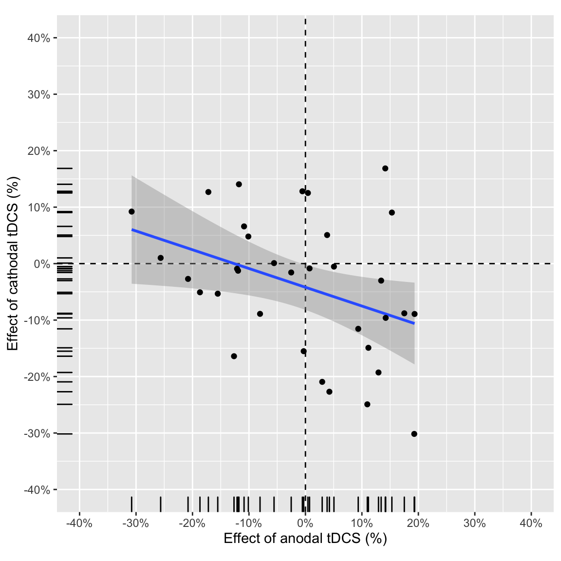
Effect of anodal vs. effect of cathodal in study 1
Study 2
plot_anodalVScathodal(ABmagChange_study2)## `geom_smooth()` using formula 'y ~ x'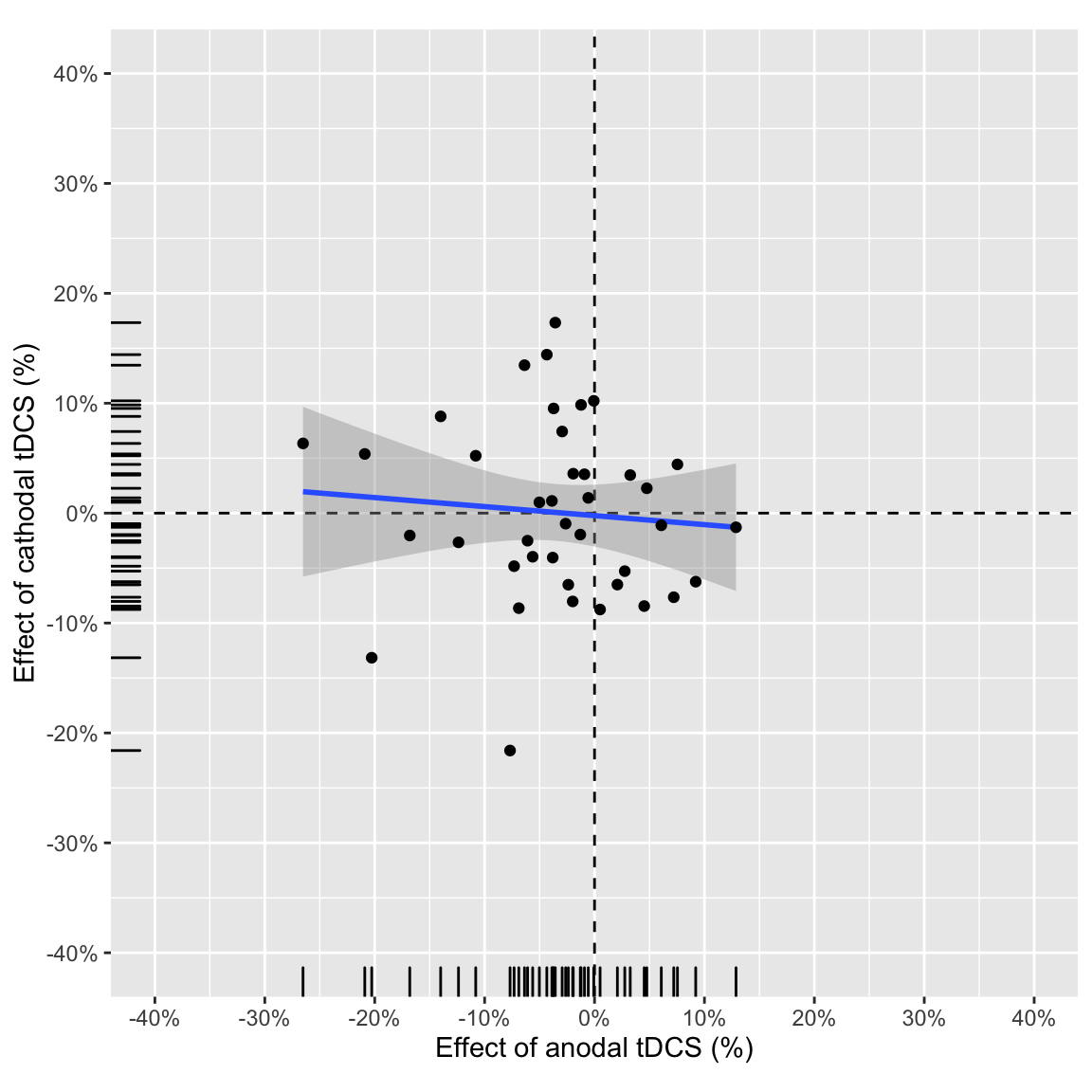
Effect of anodal vs. effect of cathodal in study 2
Statistics
pcorr_anodal_cathodal <- function(df) {
  df %>%
    # create two columns of AB magnitude change score during tDCS: for anodal and cathodal
    filter(measure == "AB.magnitude") %>%
    select(-baseline) %>%
    spread(stimulation, change.score) %>%
    ungroup() %>% # remove grouping from previous steps, as we need to modify the dataframe
    select(session.order, change, anodal, cathodal) %>% # keep only relevant columns
    mutate(session.order = as.numeric(session.order)) %>% # dummy code to use as covariate
    nest_legacy(-change) %>% # split into two data frames, one for each comparison
    # partial correlation
    mutate(r = map_dbl(data, ~pcor(c("anodal","cathodal","session.order"), var(.)))) %>%
    group_by(change) %>% # for each correlation
    # get t-stats, df and p-value of coefficient
    mutate(stats = list(as.data.frame(pcor.test(r, 1, n_distinct(df$subject))))) %>%
    unnest_legacy(stats, .drop = TRUE) # unpack resulting data frame into separate column
}
Study 1
Partial correlation between anodal and cathodal AB magnitude change score (tDCS - baseline), “controlling” for session order:
pcorr_anodal_cathodal(ABmagChange_study1) %>%
kable(digits = 3, caption = "Partial correlations study 1")| change | r | tval | df | pvalue |
|---|---|---|---|---|
| tDCS - baseline | -0.445 | -2.770 | 31 | 0.009 |
| post - baseline | 0.278 | 1.612 | 31 | 0.117 |
Zero-order correlation:
ABmagChange_study1 %>%
  ungroup() %>%
  filter(measure == "AB.magnitude") %>%
  select(-baseline) %>%
  spread(stimulation, change.score) %>%
  nest(data = -one_of('change')) %>%
  mutate(stats = map(data, ~cor.test(.$anodal, .$cathodal,
                                     alternative = "two.sided",
                                     method = "pearson"))) %>%
  mutate(stats = map(stats, tidy)) %>%
  select(-data) %>%
  unnest(stats) %>%
kable(digits = 3, caption = "zero-order correlations study 1")| change | estimate | statistic | p.value | parameter | conf.low | conf.high | method | alternative |
|---|---|---|---|---|---|---|---|---|
| tDCS - baseline | -0.376 | -2.295 | 0.028 | 32 | -0.634 | -0.043 | Pearson’s product-moment correlation | two.sided |
| post - baseline | 0.275 | 1.615 | 0.116 | 32 | -0.070 | 0.561 | Pearson’s product-moment correlation | two.sided |
Bayes factor:
ABmagChange_study1 %>%
  ungroup() %>%
  filter(measure == "AB.magnitude") %>%
  select(-baseline) %>%
  spread(stimulation, change.score) %>%
  nest_legacy(-change) %>%
  mutate(stats = map(data, ~extractBF(correlationBF(.$anodal, .$cathodal)))) %>%
  unnest_legacy(stats) %>%
  select(change, bf) %>%
kable(digits = 2, caption = "Bayesian correlations study 1")| change | bf |
|---|---|
| tDCS - baseline | 3.0 |
| post - baseline | 1.1 |
Study 2
Partial correlation between anodal and cathodal AB magnitude change score (tDCS - baseline), attempting to adjust for session order:
pcorr_anodal_cathodal(ABmagChange_study2) %>%
kable(digits = 3, caption = "Partial correlations study 2")| change | r | tval | df | pvalue |
|---|---|---|---|---|
| tDCS - baseline | 0.021 | 0.128 | 37 | 0.899 |
| post - baseline | 0.083 | 0.505 | 37 | 0.616 |
Zero-order correlation:
ABmagChange_study2 %>%
  ungroup() %>%
  filter(measure == "AB.magnitude") %>%
  select(-baseline) %>%
  spread(stimulation, change.score) %>%
  nest(data = -one_of('change')) %>%
  mutate(stats = map(data, ~cor.test(.$anodal, .$cathodal,
                                     alternative = "two.sided",
                                     method = "pearson"))) %>%
  mutate(stats = map(stats, tidy)) %>%
  select(-data) %>%
  unnest(stats) %>%
kable(digits = 3, caption = "zero-order correlations study 2")| change | estimate | statistic | p.value | parameter | conf.low | conf.high | method | alternative |
|---|---|---|---|---|---|---|---|---|
| tDCS - baseline | -0.085 | -0.525 | 0.603 | 38 | -0.386 | 0.233 | Pearson’s product-moment correlation | two.sided |
| post - baseline | -0.065 | -0.404 | 0.689 | 38 | -0.369 | 0.251 | Pearson’s product-moment correlation | two.sided |
Bayes factor:
ABmagChange_study2 %>%
  ungroup() %>%
  filter(measure == "AB.magnitude") %>%
  select(-baseline) %>%
  spread(stimulation, change.score) %>%
  nest_legacy(-change) %>%
  mutate(stats = map(data, ~extractBF(correlationBF(.$anodal, .$cathodal)))) %>%
  unnest_legacy(stats) %>%
  select(change, bf) %>%
kable(digits = 2, caption = "Bayesian correlations study 2")| change | bf |
|---|---|
| tDCS - baseline | 0.40 |
| post - baseline | 0.38 |
London, R. E., & Slagter, H. A. (2021). No Effect of Transcranial Direct Current Stimulation over Left Dorsolateral Prefrontal Cortex on Temporal Attention. Journal of Cognitive Neuroscience, 33(4), 756–768. doi: 10.1162/jocn_a_01679↩︎