Setup environment

# Load packages
library(tidyverse)  # importing, transforming, and visualizing data frames

## ── Attaching packages ─────────────────────────────────────── tidyverse 1.3.0 ──

## ✓ ggplot2 3.3.3     ✓ purrr   0.3.4
## ✓ tibble  3.0.6     ✓ dplyr   1.0.4
## ✓ tidyr   1.1.2     ✓ stringr 1.4.0
## ✓ readr   1.4.0     ✓ forcats 0.5.1

## ── Conflicts ────────────────────────────────────────── tidyverse_conflicts() ──
## x dplyr::filter() masks stats::filter()
## x dplyr::lag()    masks stats::lag()

library(here) # (relative) file paths

## here() starts at /Users/leonreteig/AB-tDCS

library(knitr) # R notebook output
library(scales) # Percentage axis labels

## 
## Attaching package: 'scales'

## The following object is masked from 'package:purrr':
## 
##     discard

## The following object is masked from 'package:readr':
## 
##     col_factor

library(afex) # analysis of factorial experiments (repeated measures anova)

## Loading required package: lme4

## Loading required package: Matrix

## 
## Attaching package: 'Matrix'

## The following objects are masked from 'package:tidyr':
## 
##     expand, pack, unpack

## Registered S3 methods overwritten by 'car':
##   method                          from
##   influence.merMod                lme4
##   cooks.distance.influence.merMod lme4
##   dfbeta.influence.merMod         lme4
##   dfbetas.influence.merMod        lme4

## ************
## Welcome to afex. For support visit: http://afex.singmann.science/

## - Functions for ANOVAs: aov_car(), aov_ez(), and aov_4()
## - Methods for calculating p-values with mixed(): 'KR', 'S', 'LRT', and 'PB'
## - 'afex_aov' and 'mixed' objects can be passed to emmeans() for follow-up tests
## - NEWS: library('emmeans') now needs to be called explicitly!
## - Get and set global package options with: afex_options()
## - Set orthogonal sum-to-zero contrasts globally: set_sum_contrasts()
## - For example analyses see: browseVignettes("afex")
## ************

## 
## Attaching package: 'afex'

## The following object is masked from 'package:lme4':
## 
##     lmer

library(emmeans); afex_options(emmeans_model = "multivariate") # post-hoc tests / contrasts, based on multivariate model
library(knitrhooks) # printing in rmarkdown outputs
  output_max_height()
# Source functions
source(here("src", "func", "behavioral_analysis.R")) # loading data and calculating measures
load_data_path <- here("src","func","load_data.Rmd") # for rerunning and displaying
knitr::read_chunk(here("src", "func", "behavioral_analysis.R")) # display code from file in this notebook

print(sessionInfo())

## R version 3.6.2 (2019-12-12)
## Platform: x86_64-apple-darwin15.6.0 (64-bit)
## Running under: macOS  10.16
## 
## Matrix products: default
## BLAS:   /Library/Frameworks/R.framework/Versions/3.6/Resources/lib/libRblas.0.dylib
## LAPACK: /Library/Frameworks/R.framework/Versions/3.6/Resources/lib/libRlapack.dylib
## 
## locale:
## [1] en_US.UTF-8/en_US.UTF-8/en_US.UTF-8/C/en_US.UTF-8/en_US.UTF-8
## 
## attached base packages:
## [1] stats     graphics  grDevices datasets  utils     methods   base     
## 
## other attached packages:
##  [1] knitrhooks_0.0.4 emmeans_1.5.4    afex_0.28-1      lme4_1.1-26     
##  [5] Matrix_1.3-2     scales_1.1.1     knitr_1.31       here_1.0.1      
##  [9] forcats_0.5.1    stringr_1.4.0    dplyr_1.0.4      purrr_0.3.4     
## [13] readr_1.4.0      tidyr_1.1.2      tibble_3.0.6     ggplot2_3.3.3   
## [17] tidyverse_1.3.0 
## 
## loaded via a namespace (and not attached):
##  [1] nlme_3.1-152        fs_1.5.0            lubridate_1.7.9.2  
##  [4] httr_1.4.2          rprojroot_2.0.2     numDeriv_2016.8-1.1
##  [7] tools_3.6.2         backports_1.2.1     R6_2.5.0           
## [10] DBI_1.1.1           colorspace_2.0-0    withr_2.4.1        
## [13] tidyselect_1.1.0    curl_4.3            compiler_3.6.2     
## [16] cli_2.3.0           rvest_0.3.6         xml2_1.3.2         
## [19] bookdown_0.21       mvtnorm_1.1-1       digest_0.6.27      
## [22] foreign_0.8-76      minqa_1.2.4         rmarkdown_2.11     
## [25] rio_0.5.26          pkgconfig_2.0.3     htmltools_0.5.1.1  
## [28] dbplyr_2.1.0        rlang_0.4.10        readxl_1.3.1       
## [31] rstudioapi_0.13     jquerylib_0.1.4     generics_0.1.0     
## [34] jsonlite_1.7.2      zip_2.1.1           car_3.0-10         
## [37] magrittr_2.0.1      Rcpp_1.0.6          munsell_0.5.0      
## [40] abind_1.4-5         lifecycle_1.0.0     stringi_1.5.3      
## [43] yaml_2.2.1          carData_3.0-4       MASS_7.3-53.1      
## [46] plyr_1.8.6          grid_3.6.2          parallel_3.6.2     
## [49] crayon_1.4.1        lattice_0.20-41     haven_2.3.1        
## [52] splines_3.6.2       hms_1.0.0           pillar_1.4.7       
## [55] boot_1.3-27         estimability_1.3    reshape2_1.4.4     
## [58] reprex_1.0.0        glue_1.4.2          evaluate_0.14      
## [61] data.table_1.13.6   renv_0.12.5-72      modelr_0.1.8       
## [64] vctrs_0.3.6         rmdformats_1.0.2    nloptr_1.2.2.2     
## [67] cellranger_1.1.0    gtable_0.3.0        assertthat_0.2.1   
## [70] xfun_0.21           openxlsx_4.2.3      xtable_1.8-4       
## [73] broom_0.7.4.9000    coda_0.19-4         lmerTest_3.1-3     
## [76] statmod_1.4.35      ellipsis_0.3.1

Load task data

Study 2

The following participants are excluded from further analysis at this point, because of incomplete data:

S03, S14, S29, S38, S43, S46: their T1 performance in session 1 was less than 63% correct, so they were not invited back. This cutoff was determined based on a separate pilot study with 10 participants. It is two standard deviations below the mean of that sample.
S25 has no data for session 2, as they stopped responding to requests for scheduling the session
S31 was excluded as a precaution after session 1, as they developed a severe headache and we could not rule out the possibility this was related to the tDCS

dataDir_study2 <- here("data") # root folder with AB task data
subs_incomplete <- c("S03", "S14", "S25", "S29", "S31", "S38", "S43", "S46") # don't try to load data from these participants
df_study2 <- load_data_study2(dataDir_study2, subs_incomplete) %>%
  filter(complete.cases(.)) %>% # discard rows with data from incomplete subjects
   # recode first.session ("anodal" or "cathodal") to session.order ("anodal first", "cathodal first")
  mutate(first.session = parse_factor(paste(first.session, "first"), 
                                      levels = c("anodal first", "cathodal first"))) %>%
  rename(session.order = first.session)
n_study2 <- n_distinct(df_study2$subject) # number of subjects in study 2

kable(head(df_study2,13), digits = 1, caption = "Data frame for study 2")

Data frame for study 2
subject	session.order	stimulation	block	lag	trials	T1	T2	T2.given.T1
S01	anodal first	anodal	pre	3	118	0.8	0.4	0.4
S01	anodal first	anodal	pre	8	60	0.8	0.8	0.8
S01	anodal first	anodal	tDCS	3	126	0.8	0.3	0.3
S01	anodal first	anodal	tDCS	8	65	0.8	0.7	0.7
S01	anodal first	anodal	post	3	122	0.8	0.2	0.3
S01	anodal first	anodal	post	8	61	0.7	0.7	0.7
S01	anodal first	cathodal	pre	3	116	0.8	0.4	0.4
S01	anodal first	cathodal	pre	8	60	0.7	0.8	0.8
S01	anodal first	cathodal	tDCS	3	129	0.7	0.4	0.4
S01	anodal first	cathodal	tDCS	8	64	0.7	0.8	0.9
S01	anodal first	cathodal	post	3	128	0.6	0.4	0.4
S01	anodal first	cathodal	post	8	62	0.7	0.8	0.8
S02	cathodal first	anodal	pre	3	124	1.0	0.8	0.8

The data has the following columns:

subject: Participant ID, e.g. S01, S12
session.order: Whether participant received anodal or cathodal tDCS in the first session (anodal_first vs. cathodal_first).
stimulation: Whether participant received anodal or cathodal tDCS
block: Whether data is before (pre), during (tDCS) or after (post`) tDCS
lag: Whether T2 followed T1 after two distractors (lag 3) or after 7 distractors (lag 8)
trials: Number of trials per lag that the participant completed in this block
T1: Proportion of trials (out of trials) in which T1 was identified correctly
T2: Proportion of trials (out of trials) in which T2 was identified correctly
T2.given.T1: Proportion of trials which T2 was identified correctly, out of the trials in which T1 was idenitified correctly (T2|T1).

The number of trials vary from person-to-person, as some completed more trials in a 20-minute block than others (because responses were self-paced):

df_study2 %>%
  group_by(lag) %>%
  summarise_at(vars(trials), funs(mean, min, max, sd)) %>%
  kable(caption = "Descriptive statistics for trial counts per lag", digits = 0)

## Warning: `funs()` was deprecated in dplyr 0.8.0.
## Please use a list of either functions or lambdas: 
## 
##   # Simple named list: 
##   list(mean = mean, median = median)
## 
##   # Auto named with `tibble::lst()`: 
##   tibble::lst(mean, median)
## 
##   # Using lambdas
##   list(~ mean(., trim = .2), ~ median(., na.rm = TRUE))

Descriptive statistics for trial counts per lag
lag	mean	min	max	sd
3	130	78	163	17
8	65	39	87	9

Study 1

These data were used for statistical analysis in London & Slagter (2021)¹, and were processed by the lead author:

dataPath_study1 <- here("data","AB-tDCS_study1.txt")
data_study1_fromDisk <- read.table(dataPath_study1, header = TRUE, dec = ",")
glimpse(data_study1_fromDisk)

## Rows: 34
## Columns: 120
## $ SD_T1                            0.3313, 0.0289, -0.8027, -0.5381, -2.…
## $ MeanBLT1Acc                      0.8800, 0.8600, 0.8050, 0.8225, 0.665…
## $ First_Session                    1, 2, 1, 1, 2, 1, 2, 1, 2, 2, 1, 2, 1…
## $ fileno                           pp4, pp6, pp7, pp9, pp10, pp11, pp12,…
## $ AB_HighLow                       2, 1, 2, 1, 1, 1, 1, 1, 2, 1, 1, 2, 1…
## $ vb_T1_2_NP                       0.925, 0.875, 0.825, 0.625, 0.650, 0.…
## $ vb_T1_4_NP                       0.800, 0.825, 0.825, 0.825, 0.675, 0.…
## $ vb_T1_10_NP                      0.925, 0.925, 0.800, 0.775, 0.825, 0.…
## $ vb_T1_4_P                        0.850, 0.900, 0.825, 0.775, 0.625, 0.…
## $ vb_T1_10_P                       0.825, 0.900, 0.775, 0.825, 0.625, 0.…
## $ vb_NB_2_NP                       0.1351, 0.3429, 0.3636, 0.3600, 0.346…
## $ vb_NB_4_NP                       0.3125, 0.5455, 0.5455, 0.3030, 0.296…
## $ vb_NB_10_NP                      0.8378, 0.8108, 0.9688, 0.6129, 0.727…
## $ vb_NB_4_P                        0.2941, 0.5278, 0.6061, 0.3226, 0.520…
## $ vb_NB_10_P                       0.8485, 0.7778, 0.9032, 0.8182, 0.680…
## $ VB_AB                            0.7027, 0.4680, 0.6051, 0.2529, 0.381…
## $ VB_REC                           0.5253, 0.2654, 0.4233, 0.3099, 0.431…
## $ VB_PE                            -0.0184, -0.0177, 0.0606, 0.0196, 0.2…
## $ tb_T1_2_NP                       0.775, 0.875, 0.675, 0.725, 0.475, 0.…
## $ tb_T1_4_NP                       0.825, 0.825, 0.700, 0.750, 0.675, 0.…
## $ tb_T1_10_NP                      0.875, 0.900, 0.700, 0.825, 0.500, 0.…
## $ tb_T1_4_P                        0.875, 0.800, 0.700, 0.775, 0.650, 0.…
## $ tb_T1_10_P                       0.850, 0.925, 0.800, 0.825, 0.625, 0.…
## $ tb_NB_2_NP                       0.1290, 0.5143, 0.2222, 0.0690, 0.315…
## $ tb_NB_4_NP                       0.3333, 0.5455, 0.6071, 0.1333, 0.370…
## $ tb_NB_10_NP                      0.8286, 0.8611, 0.8571, 0.5152, 0.850…
## $ tb_NB_4_P                        0.3143, 0.6250, 0.5357, 0.4839, 0.538…
## $ tb_NB_10_P                       0.8529, 0.7568, 0.9375, 0.6667, 0.680…
## $ TB_AB                            0.6995, 0.3468, 0.6349, 0.4462, 0.534…
## $ TB_REC                           0.4952, 0.3157, 0.2500, 0.3818, 0.479…
## $ TB_PE                            -0.0190, 0.0795, -0.0714, 0.3505, 0.1…
## $ nb_T1_2_NP                       0.850, 0.850, 0.650, 0.725, 0.675, 0.…
## $ nb_T1_4_NP                       0.800, 0.850, 0.725, 0.675, 0.575, 0.…
## $ nb_T1_10_NP                      0.925, 0.825, 0.750, 0.850, 0.725, 0.…
## $ nb_T1_4_P                        0.850, 0.900, 0.675, 0.750, 0.875, 0.…
## $ nb_T1_10_P                       0.900, 0.825, 0.750, 0.800, 0.550, 0.…
## $ nb_NB_2_NP                       0.0588, 0.4412, 0.4615, 0.1034, 0.296…
## $ nb_NB_4_NP                       0.0938, 0.4412, 0.2414, 0.1481, 0.478…
## $ nb_NB_10_NP                      0.8649, 0.7576, 0.9667, 0.6765, 0.896…
## $ nb_NB_4_P                        0.4118, 0.7222, 0.4815, 0.3667, 0.685…
## $ nb_NB_10_P                       0.8333, 0.8485, 0.8333, 0.7188, 0.818…
## $ NB_AB                            0.8060, 0.3164, 0.5051, 0.5730, 0.600…
## $ NB_REC                           0.7711, 0.3164, 0.7253, 0.5283, 0.418…
## $ NB_PE                            0.3180, 0.2810, 0.2401, 0.2185, 0.207…
## $ vd_T1_2_NP                       0.925, 0.875, 0.800, 0.850, 0.575, 0.…
## $ vd_T1_4_NP                       0.850, 0.825, 0.825, 0.925, 0.700, 0.…
## $ vd_T1_10_NP                      0.850, 0.900, 0.825, 0.925, 0.750, 0.…
## $ vd_T1_4_P                        0.925, 0.775, 0.825, 0.750, 0.650, 0.…
## $ vd_T1_10_P                       0.925, 0.800, 0.725, 0.950, 0.575, 0.…
## $ vd_NB_2_NP                       0.0541, 0.2857, 0.3125, 0.1765, 0.173…
## $ vd_NB_4_NP                       0.2941, 0.4848, 0.4545, 0.2432, 0.428…
## $ vd_NB_10_NP                      1.0000, 0.6667, 0.9394, 0.7838, 0.766…
## $ vd_NB_4_P                        0.5135, 0.6774, 0.4848, 0.5000, 0.500…
## $ vd_NB_10_P                       0.8919, 0.8125, 0.9310, 0.8421, 0.608…
## $ VD_AB                            0.9459, 0.3810, 0.6269, 0.6073, 0.592…
## $ VD_REC                           0.7059, 0.1818, 0.4848, 0.5405, 0.338…
## $ VD_PE                            0.2194, 0.1926, 0.0303, 0.2568, 0.071…
## $ td_T1_2_NP                       0.950, 0.775, 0.625, 0.775, 0.525, 0.…
## $ td_T1_4_NP                       0.975, 0.800, 0.800, 0.750, 0.625, 0.…
## $ td_T1_10_NP                      0.975, 0.900, 0.800, 0.850, 0.575, 0.…
## $ td_T1_4_P                        0.875, 0.800, 0.800, 0.800, 0.600, 0.…
## $ td_T1_10_P                       0.875, 0.800, 0.850, 0.700, 0.525, 0.…
## $ td_NB_2_NP                       0.1579, 0.3226, 0.5200, 0.1290, 0.142…
## $ td_NB_4_NP                       0.4615, 0.4375, 0.3750, 0.2333, 0.320…
## $ td_NB_10_NP                      0.9487, 0.6944, 0.9375, 0.6471, 0.826…
## $ td_NB_4_P                        0.4571, 0.3750, 0.5625, 0.4063, 0.583…
## $ td_NB_10_P                       0.8857, 0.6875, 0.8529, 0.7143, 0.666…
## $ TD_AB                            0.7908, 0.3719, 0.4175, 0.5180, 0.683…
## $ TD_REC                           0.4872, 0.2569, 0.5625, 0.4137, 0.506…
## $ TD_PE                            -0.0044, -0.0625, 0.1875, 0.1729, 0.2…
## $ nd_T1_2_NP                       0.700, 0.800, 0.650, 0.775, 0.425, 0.…
## $ nd_T1_4_NP                       0.850, 0.850, 0.725, 0.850, 0.650, 0.…
## $ nd_T1_10_NP                      0.800, 0.825, 0.800, 0.850, 0.600, 0.…
## $ nd_T1_4_P                        0.850, 0.800, 0.775, 0.775, 0.725, 0.…
## $ nd_T1_10_P                       0.850, 0.750, 0.800, 0.850, 0.675, 0.…
## $ nd_NB_2_NP                       0.0000, 0.2188, 0.2692, 0.0968, 0.235…
## $ nd_NB_4_NP                       0.3824, 0.5000, 0.5172, 0.2353, 0.384…
## $ nd_NB_10_NP                      0.8750, 0.5758, 0.8125, 0.7941, 0.708…
## $ nd_NB_4_P                        0.4118, 0.5000, 0.5806, 0.5484, 0.482…
## $ nd_NB_10_P                       0.9118, 0.7667, 0.8438, 0.8235, 0.629…
## $ ND_AB                            0.8750, 0.3570, 0.5433, 0.6973, 0.473…
## $ ND_REC                           0.4926, 0.0758, 0.2953, 0.5588, 0.323…
## $ ND_PE                            0.0294, 0.0000, 0.0634, 0.3131, 0.098…
## $ AnoMinBl_Lag2_NP                 -0.01, 0.17, -0.14, -0.29, -0.03, 0.0…
## $ AnoMinBl_Lag10_NP                -0.01, 0.05, -0.11, -0.10, 0.12, -0.0…
## $ CathoMinBl_Lag2_NP               0.10, 0.04, 0.21, -0.05, -0.03, 0.09,…
## $ CathoMinBl_Lag10_NP              -0.05, 0.03, 0.00, -0.14, 0.06, 0.00,…
## $ Tijdens_AnoMinBl_Lag2_NP         -0.01, 0.17, -0.14, -0.29, -0.03, 0.0…
## $ Tijdens_AnoMinBl_Lag10_NP        -0.01, 0.05, -0.11, -0.10, 0.12, -0.0…
## $ Tijdens_CathoMinBl_Lag2_NP       0.10, 0.04, 0.21, -0.05, -0.03, 0.09,…
## $ Tijdens_CathoMinBl_Lag10_NP      -0.05, 0.03, 0.00, -0.14, 0.06, 0.00,…
## $ Tijdens_AnoMinBL_AB              0.00, -0.12, 0.03, 0.19, 0.15, -0.08,…
## $ Tijdens_CathoMinBL_AB            -0.16, -0.01, -0.21, -0.09, 0.09, -0.…
## $ Na_AnoMinBL_AB                   0.10, -0.15, -0.10, 0.32, 0.22, -0.04…
## $ Na_CathoMinBL_AB                 -0.07, -0.02, -0.08, 0.09, -0.12, -0.…
## $ Tijdens_AnoMinBL_PE              0.00, 0.10, -0.13, 0.33, -0.06, -0.06…
## $ Tijdens_CathoMinBL_PE            -0.22, -0.26, 0.16, -0.08, 0.19, -0.0…
## $ Na_CathoMinBL_PE                 -0.19, -0.19, 0.03, 0.06, 0.03, 0.31,…
## $ Na_AnoMinBL_PE                   0.34, 0.30, 0.18, 0.20, -0.02, 0.06, …
## $ Tijdens_AnoMinBL_REC             -0.03, 0.05, -0.17, 0.07, 0.05, 0.07,…
## $ Tijdens_CathoMinBL_REC           -0.22, 0.08, 0.08, -0.13, 0.17, -0.03…
## $ Na_CathoMinBL_REC                -0.21, -0.11, -0.19, 0.02, -0.01, 0.1…
## $ Na_AnoMinBL_REC                  0.25, 0.05, 0.30, 0.22, -0.01, 0.13, …
## $ T1_Lag2_Tijdens_Ano_Min_BL_NP    -0.15, 0.00, -0.15, 0.10, -0.18, 0.00…
## $ T1_Lag2_Tijdens_Catho_Min_BL_NP  0.02, -0.10, -0.18, -0.08, -0.05, -0.…
## $ T1_Lag2_Na_Ano_Min_BL_NP         -0.08, -0.03, -0.18, 0.10, 0.03, -0.1…
## $ T1_Lag2_Na_Catho_Min_BL_NP       -0.23, -0.08, -0.15, -0.08, -0.15, -0…
## $ T1_Lag4_Tijdens_Ano_Min_BL_NP    0.02, 0.00, -0.13, -0.08, 0.00, 0.05,…
## $ T1_Lag4_Tijdens_Catho_Min_BL_NP  0.13, -0.02, -0.02, -0.18, -0.08, 0.0…
## $ T1_Lag4_Na_Catho_Min_BL_NP       0.00, 0.03, -0.10, -0.08, -0.05, 0.13…
## $ T1_Lag4_Na_Ano_Min_BL_NP         0.00, 0.03, -0.10, -0.15, -0.10, 0.02…
## $ Mean_BL_PE                       0.10, 0.09, 0.05, 0.14, 0.15, -0.13, …
## $ ZVB_AB                           0.72613, -0.71847, 0.12559, -2.04185,…
## $ ZTB_AB                           0.97738, -1.74477, 0.47867, -0.97793,…
## $ ZNB_AB                           1.24043, -1.72891, -0.58440, -0.17267…
## $ ZVD_AB                           2.47191, -1.64491, 0.14714, 0.00446, …
## $ ZTD_AB                           1.39518, -1.23661, -0.94993, -0.31845…
## $ ZND_AB                           2.00765, -1.59142, -0.29725, 0.77327,…
## $ VB_T1_Acc_                       0.87, 0.89, 0.81, 0.77, 0.68, 0.95, 0…
## $ VD_T1_Acc_                       0.90, 0.84, 0.80, 0.88, 0.65, 0.90, 0…

We’ll use only a subset of columns, with the header structure block/stim_target_lag_prime, where:

block/stim is either:
1. vb: “anodal” tDCS, “pre” block (before tDCS)
2. tb: “anodal” tDCS, “tDCS” block (during tDCS)
3. nb: “anodal” tDCS, “post” block (after tDCS)
4. vd: “cathodal” tDCS, “pre” block (before tDCS)
5. td: “cathodal” tDCS, “tDCS” block (during tDCS)
6. nd: “cathodal” tDCS, “post” block (after tDCS)
target is either:
1. T1 (T1 accuracy): proportion of trials in which T1 was identified correctly
2. NB (T2|T1 accuracy): proportion of trials in which T2 was identified correctly, given T1 was identified correctly
lag is either:
1. 2 (lag 2), when T2 followed T1 after 1 distractor
2. 4 (lag 4), when T2 followed T1 after 3 distractors
3. 10, (lag 10), when T2 followed T1 after 9 distractors
prime is either:
1. P (prime): when the stimulus at lag 2 (in lag 4 or lag 10 trials) had the same identity as T2
2. NP (no prime) when this was not the case. Study 2 had no primes, so we’ll only keep these.

We’ll also keep two more columns: fileno (participant ID) and First_Session (1 meaning participants received anodal tDCS in the first session, 2 meaning participants received cathodal tDCS in the first session).

Reformat

Now we’ll reformat the data to match the data frame for study 2:

format_study2 <- function(df) {
  df %>%
    select(fileno, First_Session, ends_with("_NP"), -contains("Min")) %>% # keep only relevant columns
    gather(key, accuracy, -fileno, -First_Session) %>% # make long form
    # split key column to create separate columns for each factor
    separate(key, c("block", "stimulation", "target", "lag"), c(1,3,5)) %>% # split after 1st, 3rd, and 5th character
    # convert to factors, relabel levels to match those in study 2
    mutate(block = factor(block, levels = c("v", "t", "n"), labels = c("pre", "tDCS", "post")),
           stimulation = factor(stimulation, levels = c("b_", "d_"), labels = c("anodal", "cathodal")),
           lag = factor(lag, levels = c("_2_NP", "_4_NP", "_10_NP"), labels = c(2, 4, 10)),
           First_Session = factor(First_Session, labels = c("anodal first","cathodal first"))) %>%
    spread(target, accuracy) %>% # create separate columns for T2.given.T1 and T1 performance
    rename(T2.given.T1 = NB, session.order = First_Session, subject = fileno)# rename columns to match those in study 2
}

df_study1 <- format_study2(data_study1_fromDisk)
n_study1 <- n_distinct(df_study1$subject) # number of subjects in study 1

kable(head(df_study1,19), digits = 1, caption = "Data frame for study 1")

Data frame for study 1
subject	session.order	block	stimulation	lag	T2.given.T1	T1
pp10	cathodal first	pre	anodal	2	0.3	0.6
pp10	cathodal first	pre	anodal	4	0.3	0.7
pp10	cathodal first	pre	anodal	10	0.7	0.8
pp10	cathodal first	pre	cathodal	2	0.2	0.6
pp10	cathodal first	pre	cathodal	4	0.4	0.7
pp10	cathodal first	pre	cathodal	10	0.8	0.8
pp10	cathodal first	tDCS	anodal	2	0.3	0.5
pp10	cathodal first	tDCS	anodal	4	0.4	0.7
pp10	cathodal first	tDCS	anodal	10	0.8	0.5
pp10	cathodal first	tDCS	cathodal	2	0.1	0.5
pp10	cathodal first	tDCS	cathodal	4	0.3	0.6
pp10	cathodal first	tDCS	cathodal	10	0.8	0.6
pp10	cathodal first	post	anodal	2	0.3	0.7
pp10	cathodal first	post	anodal	4	0.5	0.6
pp10	cathodal first	post	anodal	10	0.9	0.7
pp10	cathodal first	post	cathodal	2	0.2	0.4
pp10	cathodal first	post	cathodal	4	0.4	0.6
pp10	cathodal first	post	cathodal	10	0.7	0.6
pp11	anodal first	pre	anodal	2	0.5	1.0

Group analysis

Line plots cf. London & Slagter (2021)

plot_lines <- function(df) {
  df %>%
  gather(target, proportion_correct, T1, T2.given.T1) %>% # so T1 vs. T2|T1 can be used as a factor
  
  ggplot(aes(lag, proportion_correct, color = block, linetype = target)) +
  facet_wrap(~stimulation) +
  stat_summary(fun.y = mean, geom = "line", aes(group = interaction(target,block)), position = position_dodge(width = 0.2)) +
  stat_summary(fun.data = mean_se, geom = "errorbar", position = position_dodge(width = 0.2)) +
  scale_x_discrete("Lag") +
  scale_y_continuous("Percentage correct", limits = c(0,1), breaks = seq(0,1,.1), labels = scales::percent_format())
}

Study 1

plot_lines(df_study1)

## Warning: `fun.y` is deprecated. Use `fun` instead.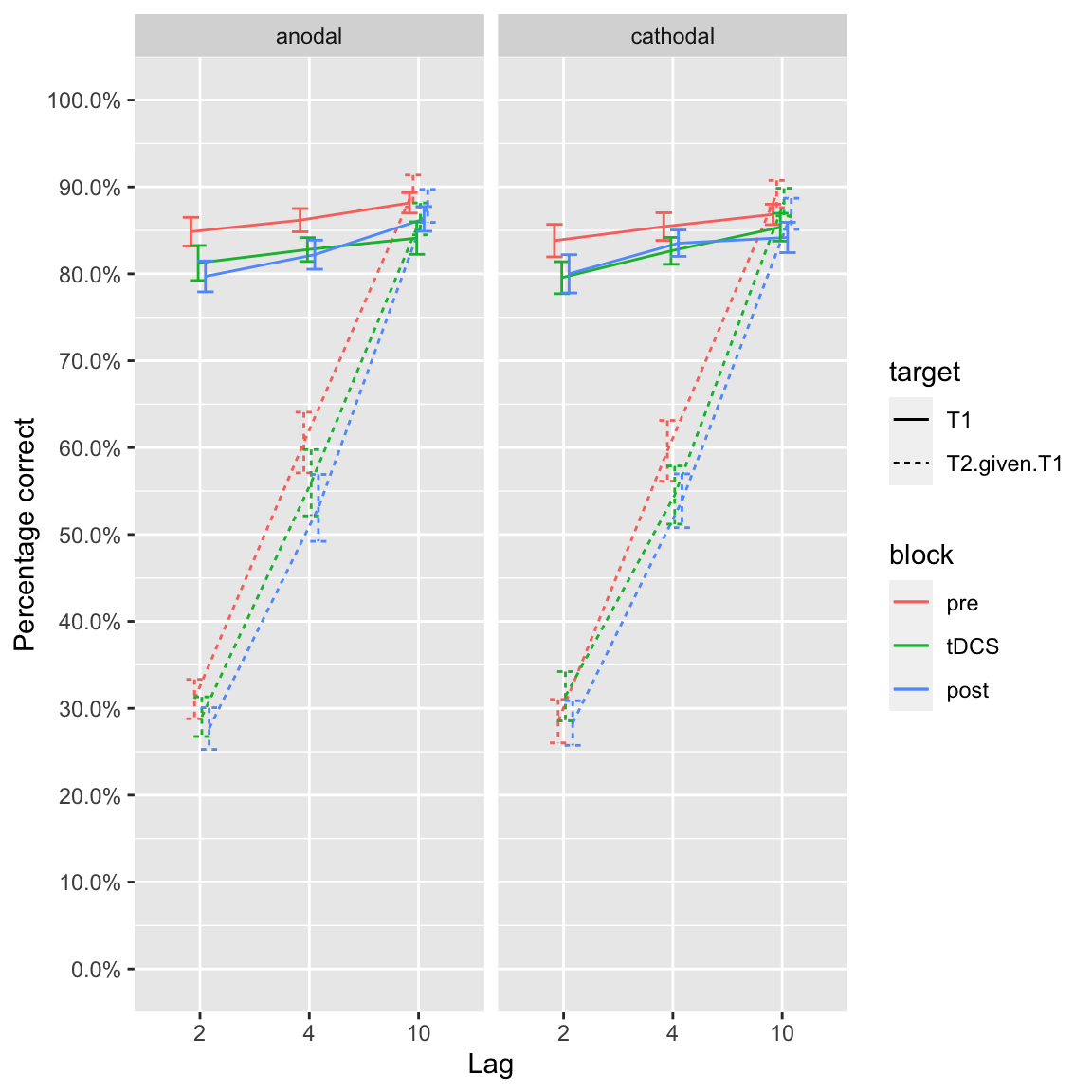

Group effects of tDCS in study 1

Study 2

plot_lines(df_study2)

## Warning: `fun.y` is deprecated. Use `fun` instead.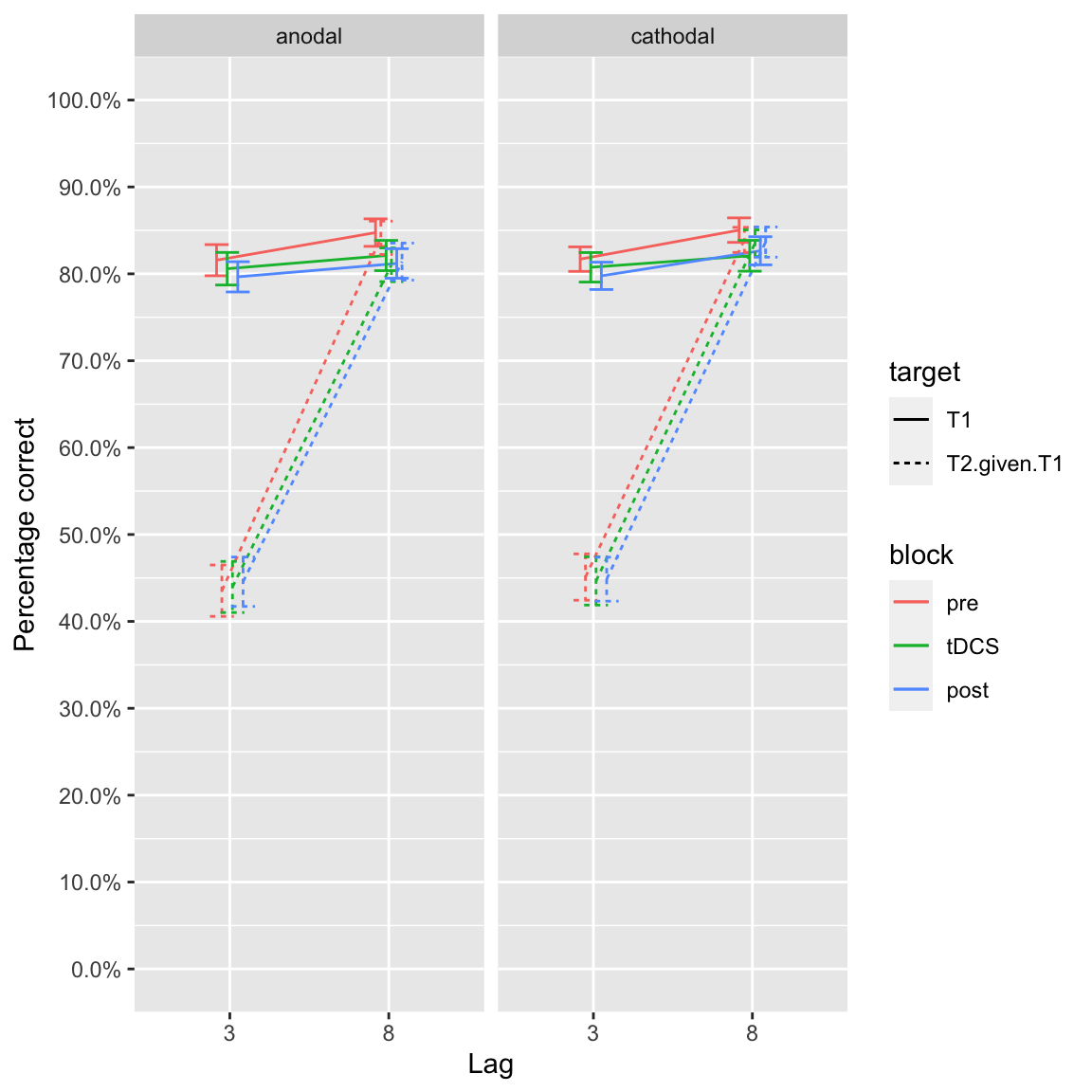

Group effects of tDCS in study 2

Stray observations:

T1 performance comparable between both studies
Lag 8 performance is comparable to lag 10 (although a little bit lower)
Blink at lag 3 is about 10-15 percentage points less than lag 2
Slopes differ a bit in study 1, in study 2 especially anodal tDCS lag 8 stands out
In both studies, performance at lag 2/3 across anodal/cathodal tDCS and blocks is basically identical

RM ANOVA

Study 1 - T2|T1

DV: T2.given.T1: Proportion of trials which T2 was identified correctly, out of the trials in which T1 was idenitified correctly (T2|T1).
Between-subject factor: session.order, 2 levels: Whether participant received anodal or cathodal tDCS in the first session (anodal_first vs. cathodal_first).
Within-subject factors:
1. block, 3 levels: Whether data is before (pre), during (tDCS) or after (post) tDCS
2. stimulation, 2 levels: Whether participant received anodal or cathodal tDCS
3. lag, 3 levels: Whether T2 followed T1 after 1 distractor (lag 2), 3 distractors, (lag 4), or after 9 distractors (lag 10).
Subject identifier: subject (n = 34).

aov_study1 <- aov_car(T2.given.T1 ~ session.order + Error(subject/(block*stimulation*lag)), 
        data = df_study1)

## Contrasts set to contr.sum for the following variables: session.order

kable(nice(aov_study1), caption = "Study 1: RM ANOVA on T2|T1 performance")

Study 1: RM ANOVA on T2|T1 performance
Effect	df	MSE	F	ges	p.value
session.order	1, 32	0.23	0.06	<.001	.812
block	1.89, 60.49	0.01	9.14 ***	.009	<.001
session.order:block	1.89, 60.49	0.01	1.99	.002	.148
stimulation	1, 32	0.01	0.18	<.001	.670
session.order:stimulation	1, 32	0.01	17.05 ***	.012	<.001
lag	1.89, 60.35	0.06	311.79 ***	.709	<.001
session.order:lag	1.89, 60.35	0.06	0.77	.006	.460
block:stimulation	1.81, 58.01	0.01	1.50	.001	.232
session.order:block:stimulation	1.81, 58.01	0.01	5.25 **	.004	.010
block:lag	3.43, 109.90	0.01	3.66 *	.005	.011
session.order:block:lag	3.43, 109.90	0.01	1.54	.002	.203
stimulation:lag	1.44, 46.15	0.01	0.05	<.001	.905
session.order:stimulation:lag	1.44, 46.15	0.01	3.48 +	.004	.053
block:stimulation:lag	3.35, 107.08	0.01	0.83	.001	.492
session.order:block:stimulation:lag	3.35, 107.08	0.01	0.70	.001	.567

Main effect of lag

This is the attentional blink: T2 is seen more often in the long lag(s).

afex_plot(aov_study1, x = "lag", error = "within")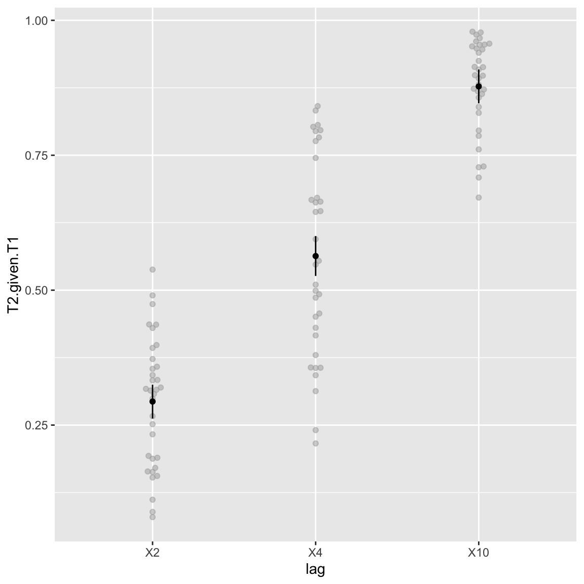

Study 1 - Attentional blink (main effect of Lag)

Main effect of block

afex_plot(aov_study1, x = "block", error = "within")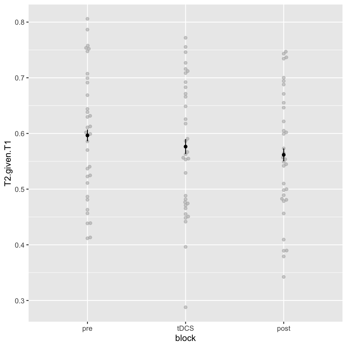

Study 1 - main effect of Block

Appears to be a time-on-task / fatigue effect: participants get worse each block.

Interaction: block by stimulation by lag

The hypothesized effect was that anodal stimulation improves (compared to pre block) the attentional blink (short-lag T2 performance), but it was not significant.

afex_plot(aov_study1, x = "block", trace =  "stimulation", panel = "lag", 
          factor_levels = list(lag = c("lag 2","lag 4","lag 10")), error = "within")

## Renaming/reordering factor levels of 'lag':
##   X2 -> lag 2
##   X4 -> lag 4
##   X10 -> lag 10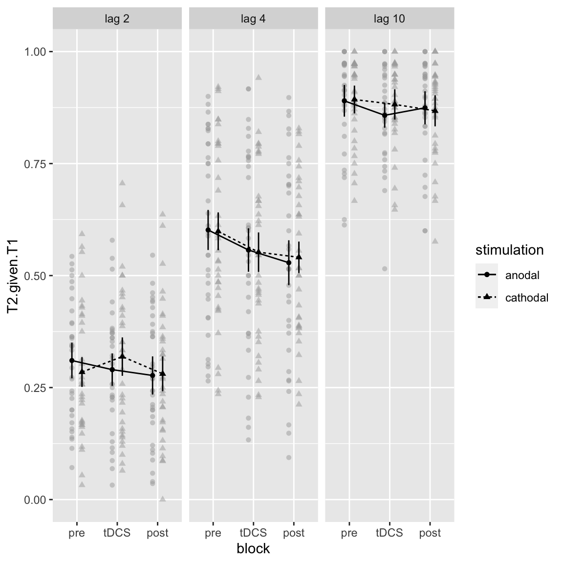

Study 1 - hypothesized interaction: Block by Stimulation by Lag

Indeed, only a main effect of lag is clearly visible. If anything, the largest difference is in lag 2 though, but in the opposite direction (cathodal slightly improves performance; anodal slightly decreases performance).

Interaction: stimulation by session order

afex_plot(aov_study1, x = "stimulation", trace = "session.order", error = "none")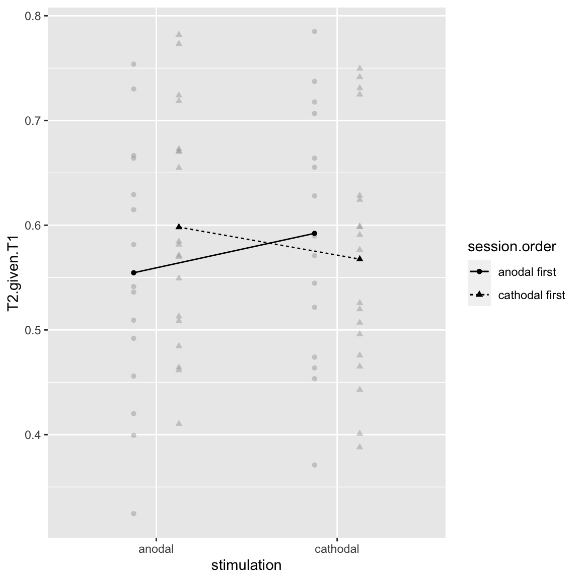

Study 1 - Stimulation by Session Order

stimulation and session.order are not orthogonal: their interaction makes up a new factor session, with 2 levels:

session 1:
1. session.order = anodal first, stimulation = anodal
2. session.order = cathodal first, stimulation = cathodal
session 2:
1. session.order = anodal first, stimulation = cathodal
2. session.order = cathodal first, stimulation = anodal

So my take is this “interaction” actually reflects an across-session learning effect: participants simply do better in their 2nd session than in their 1st.

Interaction: stimulation by session order by block

There is apparently also a higher order interaction, with block:

afex_plot(aov_study1, x = "stimulation", trace = "session.order", panel = "block", error = "none")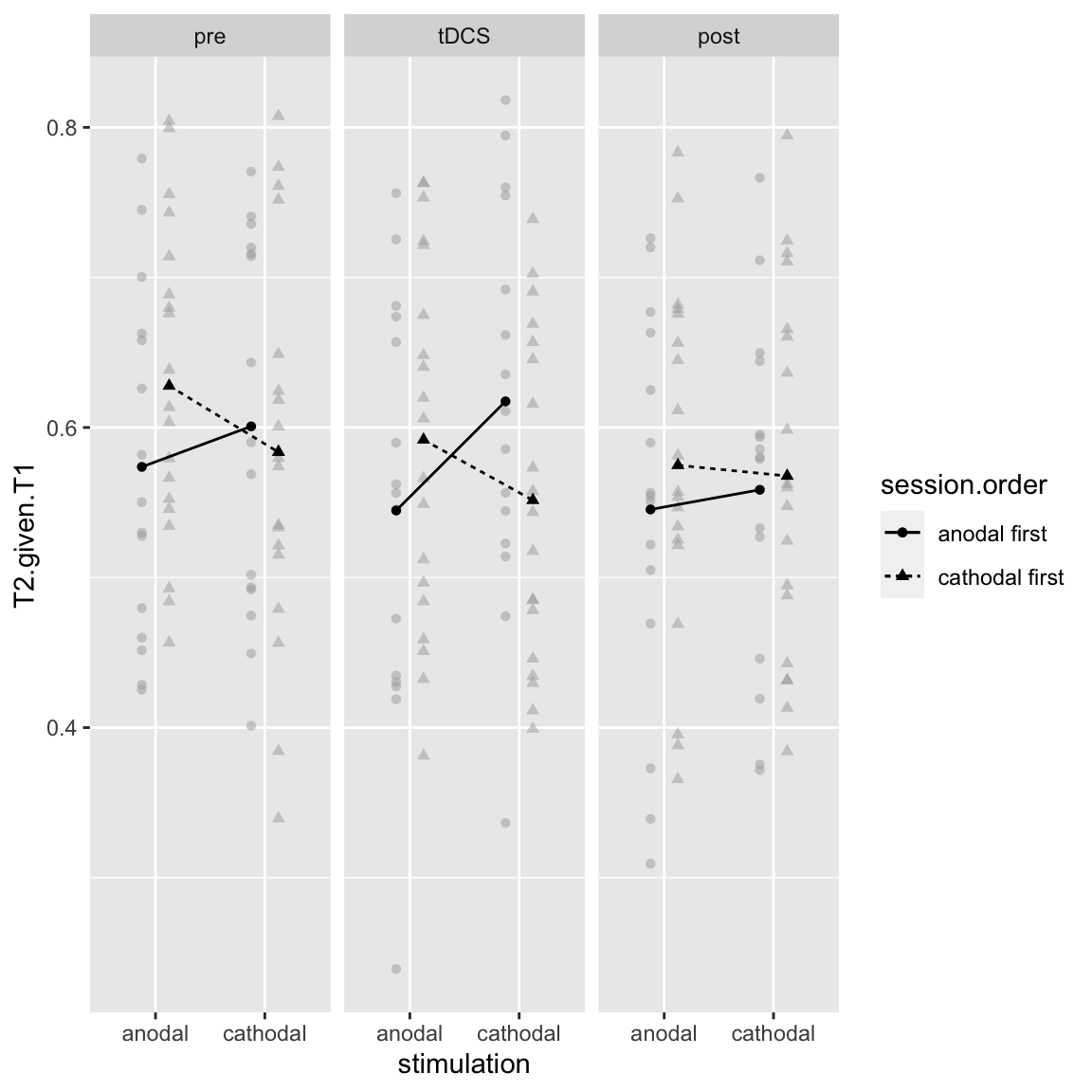

Study 1 - Stimulation by Session Order by Block

Seems that the crossover interaction (the learning effect) is mostly present in the first two blocks, not the last. This makes sense intuitively: in the third block of the 1st session, participants already performed the task for 40 minutes, so the difference in “time-on-task” between session 1 and 2 is not so great.

Study 2 - T2|T1

DV: T2.given.T1: Proportion of trials which T2 was identified correctly, out of the trials in which T1 was idenitified correctly (T2|T1).
Within-subject factors:
1. block, 3 levels: Whether data is before (pre), during (tDCS) or after (post) tDCS
2. stimulation, 2 levels: Whether participant received anodal or cathodal tDCS
3. lag, 2 levels: Whether T2 followed T1 after 2 distractors (lag 3), or after 7 distractors (lag 8).
Subject identifier: subject (n = 40).

aov_study2 <- aov_car(T2.given.T1 ~ session.order + Error(subject/(block*stimulation*lag)), 
        data = df_study2)

## Contrasts set to contr.sum for the following variables: session.order

kable(nice(aov_study2), caption = "Study 2: RM ANOVA on T2|T1 performance")

Study 2: RM ANOVA on T2|T1 performance
Effect	df	MSE	F	ges	p.value
session.order	1, 38	0.19	0.33	.006	.568
block	1.91, 72.71	0.00	1.13	<.001	.328
session.order:block	1.91, 72.71	0.00	0.29	<.001	.741
stimulation	1, 38	0.01	2.47	.002	.125
session.order:stimulation	1, 38	0.01	5.55 *	.005	.024
lag	1, 38	0.04	432.11 ***	.634	<.001
session.order:lag	1, 38	0.04	0.48	.002	.494
block:stimulation	1.91, 72.51	0.00	0.28	<.001	.747
session.order:block:stimulation	1.91, 72.51	0.00	1.93	<.001	.154
block:lag	1.70, 64.73	0.00	1.67	<.001	.199
session.order:block:lag	1.70, 64.73	0.00	0.24	<.001	.752
stimulation:lag	1, 38	0.00	0.10	<.001	.751
session.order:stimulation:lag	1, 38	0.00	5.84 *	.002	.021
block:stimulation:lag	1.77, 67.17	0.00	2.77 +	.001	.076
session.order:block:stimulation:lag	1.77, 67.17	0.00	7.25 **	.003	.002

Main effect of lag

afex_plot(aov_study2, x = "lag", error = "within")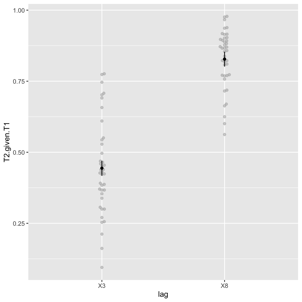

Study 2 - Attentional blink (main effect of Lag)

Again simply the attentional blink.

Interaction: block by stimulation by lag

Like in study 1, this was the hypothesized effect, but it is not significant.

afex_plot(aov_study2, x = "block", trace =  "stimulation", 
          panel = "lag", factor_levels = list(lag = c("lag 3","lag 8")), error = "within")

## Renaming/reordering factor levels of 'lag':
##   X3 -> lag 3
##   X8 -> lag 8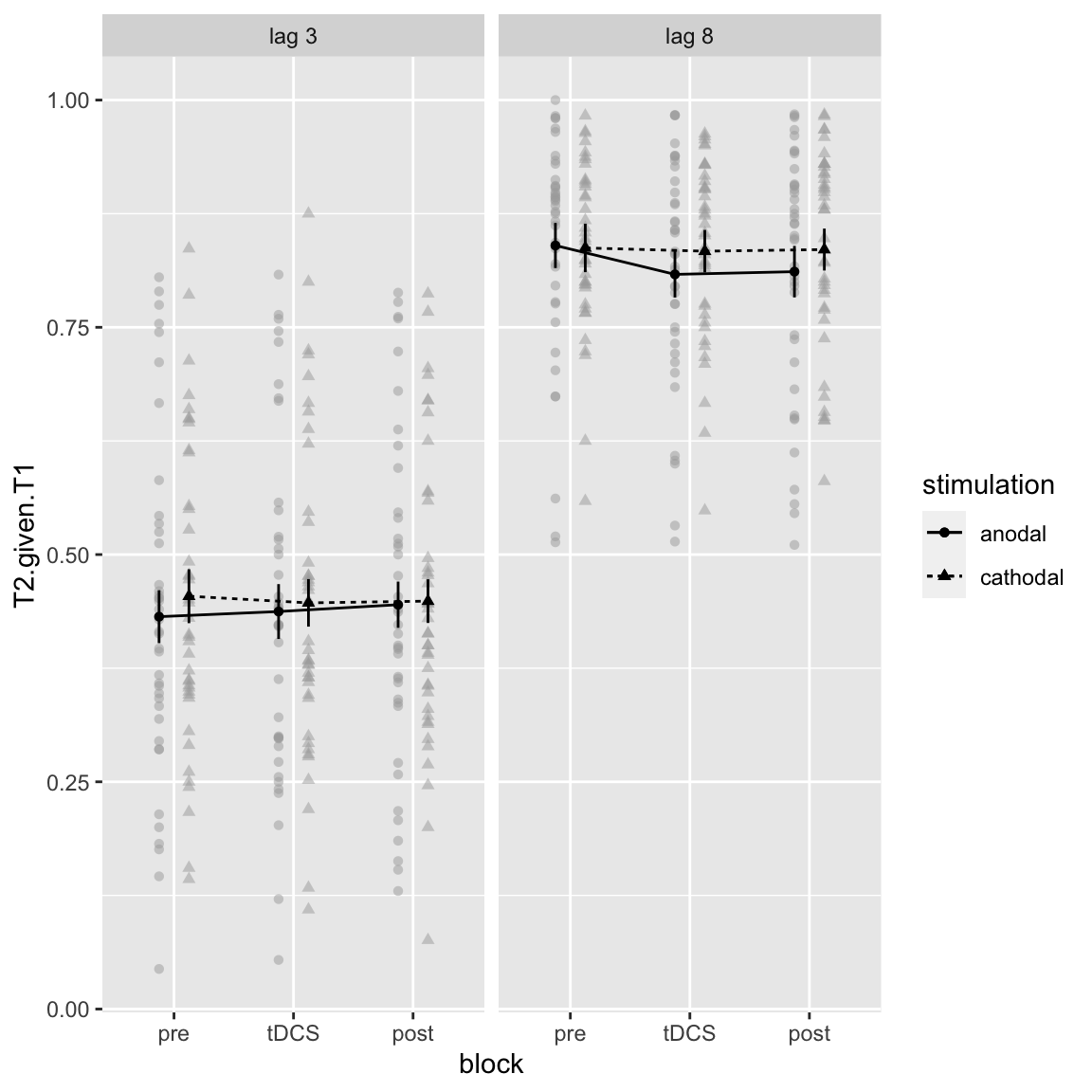

Study 2 - hypothesized interaction: Block by Stimulation by Lag

Doesn’t look like much, but as it’s trending (p = 0.076), let’s look at the contrasts anyway:

pairs(emmeans(aov_study2, ~block|stimulation*lag))

## stimulation = anodal, lag = X3:
##  contrast    estimate      SE df t.ratio p.value
##  pre - tDCS  -0.00566 0.01140 38 -0.497  0.8733 
##  pre - post  -0.01318 0.01086 38 -1.214  0.4527 
##  tDCS - post -0.00751 0.01262 38 -0.596  0.8233 
## 
## stimulation = cathodal, lag = X3:
##  contrast    estimate      SE df t.ratio p.value
##  pre - tDCS   0.00732 0.01072 38  0.683  0.7749 
##  pre - post   0.00542 0.01093 38  0.495  0.8740 
##  tDCS - post -0.00191 0.00963 38 -0.198  0.9787 
## 
## stimulation = anodal, lag = X8:
##  contrast    estimate      SE df t.ratio p.value
##  pre - tDCS   0.03180 0.00929 38  3.423  0.0042 
##  pre - post   0.02878 0.01295 38  2.222  0.0803 
##  tDCS - post -0.00302 0.01237 38 -0.244  0.9678 
## 
## stimulation = cathodal, lag = X8:
##  contrast    estimate      SE df t.ratio p.value
##  pre - tDCS   0.00356 0.01050 38  0.339  0.9387 
##  pre - post   0.00179 0.01183 38  0.151  0.9875 
##  tDCS - post -0.00178 0.01099 38 -0.162  0.9857 
## 
## Results are averaged over the levels of: session.order 
## P value adjustment: tukey method for comparing a family of 3 estimates

The only significant change is in the anodal, lag 8 condition: T2 performance goes down compared to baseline. But because this is not the case for the short lag, this should not be considered an effect on the attentional blink.

Interaction: stimulation by session order

afex_plot(aov_study2, x = "stimulation", trace = "session.order", error = "none")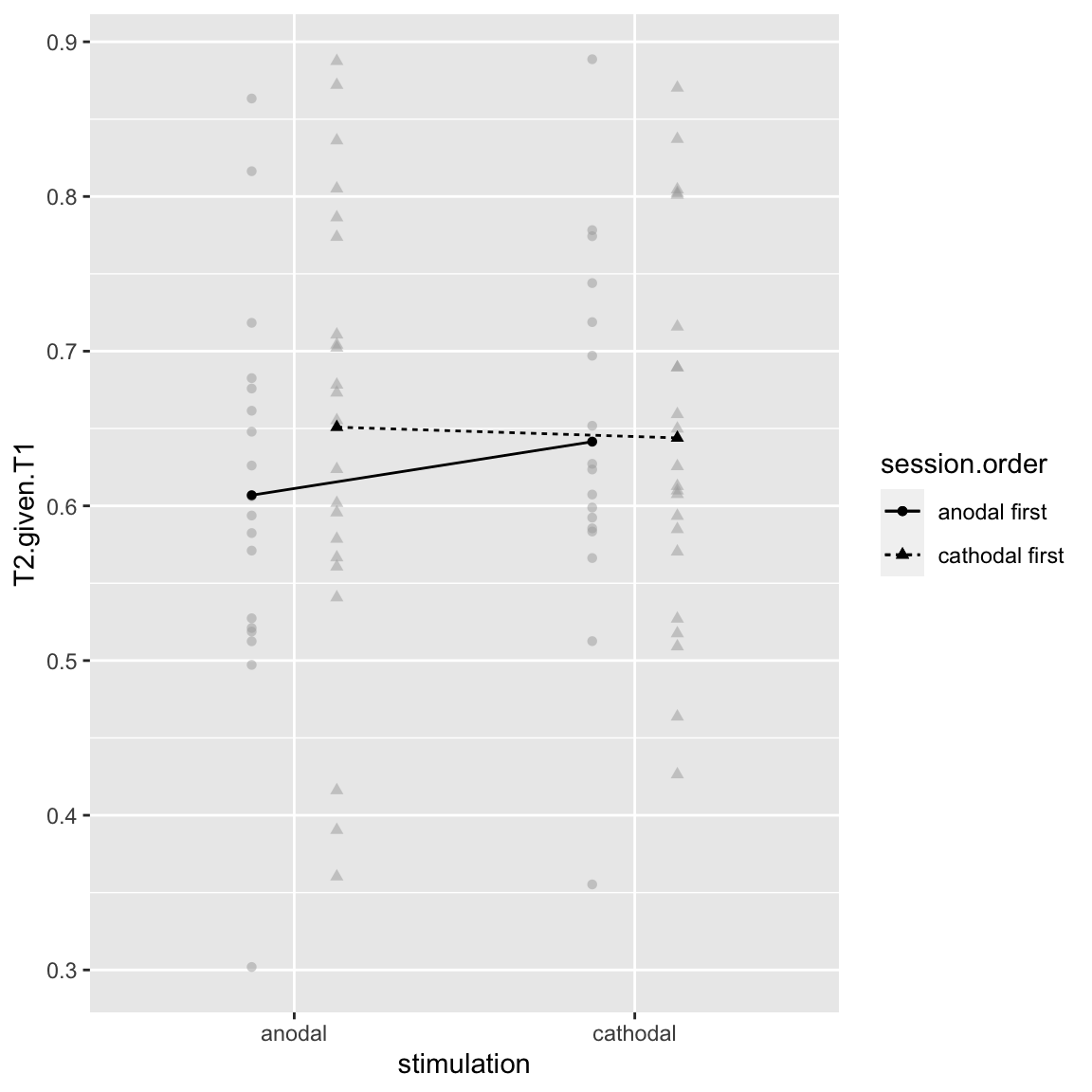

Study 2 - Stimulation by Session Order

In study 1, this interaction also occured and looked like a cross-session learning effect: performance improves in the 2nd session compared to the first. However, here this is only visible for the “anodal first” group.

pairs(emmeans(aov_study2, ~stimulation|session.order))

## session.order = anodal first:
##  contrast          estimate     SE df t.ratio p.value
##  anodal - cathodal -0.03461 0.0131 38 -2.648  0.0117 
## 
## session.order = cathodal first:
##  contrast          estimate     SE df t.ratio p.value
##  anodal - cathodal  0.00693 0.0118 38  0.586  0.5613 
## 
## Results are averaged over the levels of: lag, block

Indeed, the difference is only significant for the “anodal first” group. It’s unlikely, but in principle this could indicate that anodal has a carryover effect, while cathodal does not.

Interaction: stimulation by session order by lag

Apparently this also interacts with Lag (which it also did not do in study 1):

afex_plot(aov_study2, x = "stimulation", trace = "session.order", panel = "lag", 
          factor_levels = list(lag = c("lag 3","lag 8")), error = "none")

## Renaming/reordering factor levels of 'lag':
##   X3 -> lag 3
##   X8 -> lag 8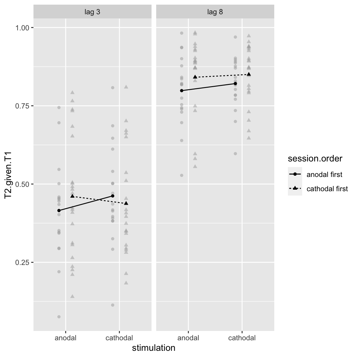

Study 2 - Stimulation by Session Order by Lag

Interesting: the two-way interaction between stimulation and session order shows no learning effect for both groups (only anodal first). However, this higher-order interaction does seem to show a change in the cathodal group also. But the interaction is only visible in the the short lag condition. That makes sense, as there is not much room for improvement in the long lag condition.

Interaction: stimulation by session order by lag by block

Then, there is a yet higher order interaction, also with block:

afex_plot(aov_study2, x = "stimulation", trace = c("session.order","lag"), 
          panel = "block", data_plot = FALSE, factor_levels = list(lag = c("lag 3","lag 8")), error = "none")

## Renaming/reordering factor levels of 'lag':
##   X3 -> lag 3
##   X8 -> lag 8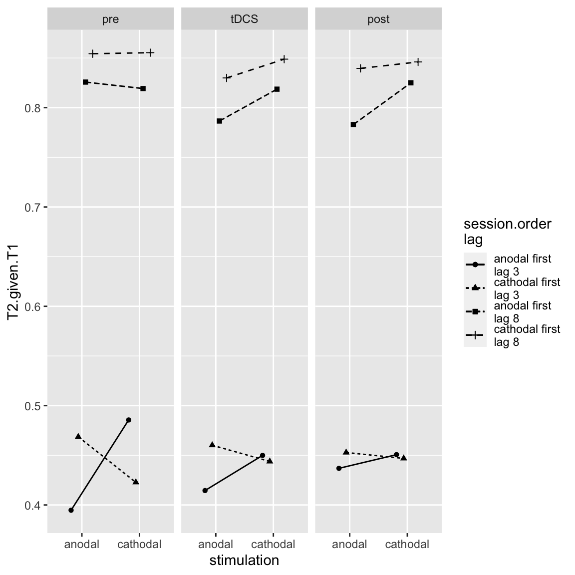

Study 2 - four way interaction, centered on Block

This suggests that the three-way interaction (cross-session learning effect for short lag) mostly occurs in the pre block. Similar to the three-way interaction in study 1 (stimulation by session order by block), the “learning effect across sessions” (crossover in short lag trials) diminishes over blocks. This makes sense because the difference between sessions in “task experience” also diminishes over blocks (in the pre block, participants are doing the task for the first time in session 1, but in the later blocks of session 1, they’ve built up experience).

However, another take on the four-way interaction is the following: it is actually the hypothesized effect (three-way interaction of stimulation, block, and lag), but it only occurs for a certain session order:

afex_plot(aov_study2, x = "block", trace = c("stimulation","lag"), panel = "session.order", data_plot = FALSE,
          factor_levels = list(lag = c("lag 3","lag 8")), error = "none")

## Renaming/reordering factor levels of 'lag':
##   X3 -> lag 3
##   X8 -> lag 8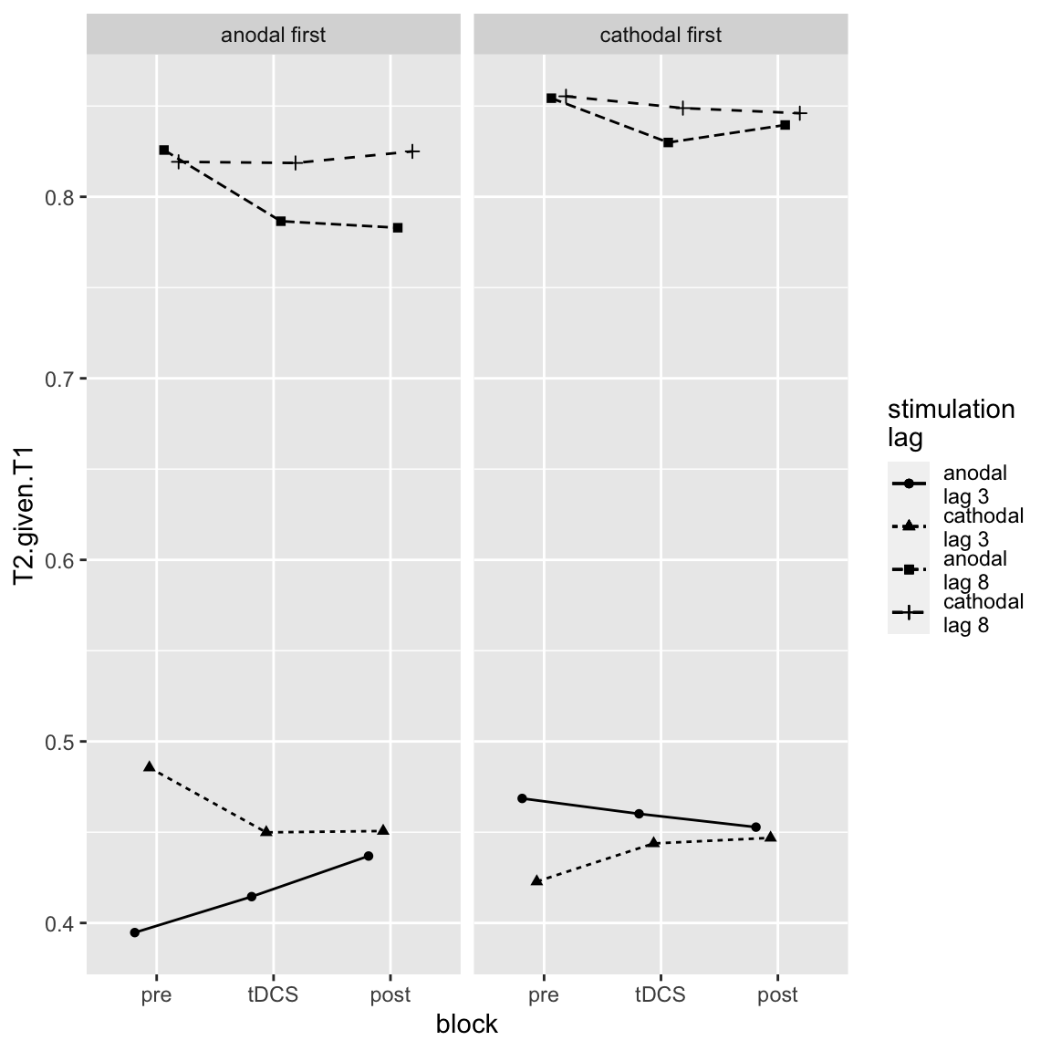

Study 2 - four way interaction, centered on Session Order

Most of the changes occur in the “anodal first” group. There we can actually see the hypothesized effect: increased performance on short-lag trials during/after tDCS compared to before. That said, the biggest difference between anodal and cathodal is in the baseline already, and only decreases in the tDCS- and post-blocks. Also, in the “cathodal first” group, the direction of the “effect” is reversed (and again the differences are largest in the baseline).

Still, lets’s look at the hypothesized three-way interaction separately for each “group” (anodal first, cathodal first):

joint_tests(aov_study2, by = "session.order")

## session.order = anodal first:
##  model term            df1 df2 F.ratio p.value
##  lag                     1  38 183.573 <.0001 
##  stimulation             1  38   7.009 0.0117 
##  block                   2  38   0.956 0.3935 
##  lag:stimulation         1  38   1.998 0.1656 
##  lag:block               2  38   0.958 0.3926 
##  stimulation:block       2  38   0.372 0.6920 
##  lag:stimulation:block   2  38  10.938 0.0002 
## 
## session.order = cathodal first:
##  model term            df1 df2 F.ratio p.value
##  lag                     1  38 256.284 <.0001 
##  stimulation             1  38   0.343 0.5613 
##  block                   2  38   0.149 0.8624 
##  lag:stimulation         1  38   4.163 0.0483 
##  lag:block               2  38   1.833 0.1738 
##  stimulation:block       2  38   1.642 0.2070 
##  lag:stimulation:block   2  38   0.684 0.5106

Indeed, so the three-way interaction is significant in the “anodal first” group, but not the “cathodal first” group.

Finally, let’s also look at the pairwise contrasts for block for each combination of factors:

pairs(emmeans(aov_study2, ~block|session.order*stimulation*lag))

## session.order = anodal first, stimulation = anodal, lag = X3:
##  contrast     estimate     SE df t.ratio p.value
##  pre - tDCS  -0.019799 0.0169 38 -1.171  0.4775 
##  pre - post  -0.042161 0.0161 38 -2.617  0.0331 
##  tDCS - post -0.022361 0.0187 38 -1.195  0.4635 
## 
## session.order = cathodal first, stimulation = anodal, lag = X3:
##  contrast     estimate     SE df t.ratio p.value
##  pre - tDCS   0.008471 0.0153 38  0.554  0.8451 
##  pre - post   0.015803 0.0146 38  1.085  0.5293 
##  tDCS - post  0.007332 0.0169 38  0.433  0.9021 
## 
## session.order = anodal first, stimulation = cathodal, lag = X3:
##  contrast     estimate     SE df t.ratio p.value
##  pre - tDCS   0.035659 0.0159 38  2.242  0.0770 
##  pre - post   0.034916 0.0162 38  2.153  0.0927 
##  tDCS - post -0.000743 0.0143 38 -0.052  0.9985 
## 
## session.order = cathodal first, stimulation = cathodal, lag = X3:
##  contrast     estimate     SE df t.ratio p.value
##  pre - tDCS  -0.021017 0.0144 38 -1.461  0.3209 
##  pre - post  -0.024085 0.0147 38 -1.642  0.2408 
##  tDCS - post -0.003068 0.0129 38 -0.237  0.9694 
## 
## session.order = anodal first, stimulation = anodal, lag = X8:
##  contrast     estimate     SE df t.ratio p.value
##  pre - tDCS   0.039205 0.0138 38  2.845  0.0190 
##  pre - post   0.042806 0.0192 38  2.228  0.0792 
##  tDCS - post  0.003601 0.0183 38  0.196  0.9790 
## 
## session.order = cathodal first, stimulation = anodal, lag = X8:
##  contrast     estimate     SE df t.ratio p.value
##  pre - tDCS   0.024392 0.0125 38  1.957  0.1369 
##  pre - post   0.014759 0.0174 38  0.849  0.6751 
##  tDCS - post -0.009633 0.0166 38 -0.581  0.8312 
## 
## session.order = anodal first, stimulation = cathodal, lag = X8:
##  contrast     estimate     SE df t.ratio p.value
##  pre - tDCS   0.000626 0.0156 38  0.040  0.9991 
##  pre - post  -0.005752 0.0175 38 -0.328  0.9426 
##  tDCS - post -0.006378 0.0163 38 -0.391  0.9193 
## 
## session.order = cathodal first, stimulation = cathodal, lag = X8:
##  contrast     estimate     SE df t.ratio p.value
##  pre - tDCS   0.006495 0.0141 38  0.461  0.8898 
##  pre - post   0.009322 0.0159 38  0.587  0.8278 
##  tDCS - post  0.002826 0.0147 38  0.192  0.9800 
## 
## P value adjustment: tukey method for comparing a family of 3 estimates

The pre - post contrast for lag 3, anodal stimulation in the anodal-first group is indeed significant (but the pre - tDCS difference is not). There is also an effect for lag 8, the pre - tDCS contrast is significant there (but not pre - post).

However, all in all, I favor the 1st interpretation of the four-way interaction (i.e. in terms of the learning effect, which does not occur at lag 8):

It’s more consistent with study 1 (also occurs there, albeit in slightly different form)
Unless there’s really a carryover effect, it’s not clear why the hypothesized effect would only occur in the “anodal first” group. A learning effect seems more intuitive.
The differences between the two stimulation sessions (anodal and cathodal) are most pronounced before tDCS onset.

Study 2 - T1

DV: T1: Proportion of trials in which T1 was identified correctly.
Between-subject factor: session.order, 2 levels: Whether participant received anodal or cathodal tDCS in the first session (anodal_first vs. cathodal_first).
Within-subject factors:
1. block, 3 levels: Whether data is before (pre), during (tDCS) or after (post) tDCS
2. stimulation, 2 levels: Whether participant received anodal or cathodal tDCS
3. lag, 2 levels: Whether T2 followed T1 after 2 distractors (lag 3), or after 7 distractors (lag 8).
Subject identifier: subject (n = 40).

aov_study2_T1 <- aov_car(T1 ~ session.order + Error(subject/(block*stimulation*lag)), 
        data = df_study2)

## Contrasts set to contr.sum for the following variables: session.order

kable(nice(aov_study2_T1), caption = "Study 2: RM ANOVA on T1 performance")

Study 2: RM ANOVA on T1 performance
Effect	df	MSE	F	ges	p.value
session.order	1, 38	0.09	0.96	.018	.332
block	1.89, 71.87	0.00	6.64 **	.010	.003
session.order:block	1.89, 71.87	0.00	0.60	<.001	.540
stimulation	1, 38	0.01	0.00	<.001	.996
session.order:stimulation	1, 38	0.01	11.24 **	.030	.002
lag	1, 38	0.00	29.23 ***	.013	<.001
session.order:lag	1, 38	0.00	0.04	<.001	.844
block:stimulation	1.92, 73.08	0.00	0.24	<.001	.777
session.order:block:stimulation	1.92, 73.08	0.00	9.94 ***	.007	<.001
block:lag	1.93, 73.20	0.00	1.91	.001	.158
session.order:block:lag	1.93, 73.20	0.00	0.19	<.001	.821
stimulation:lag	1, 38	0.00	0.31	<.001	.584
session.order:stimulation:lag	1, 38	0.00	0.96	<.001	.333
block:stimulation:lag	1.86, 70.75	0.00	0.31	<.001	.718
session.order:block:stimulation:lag	1.86, 70.75	0.00	0.53	<.001	.580

Main effect of lag

afex_plot(aov_study2_T1, x = "lag", error = "within")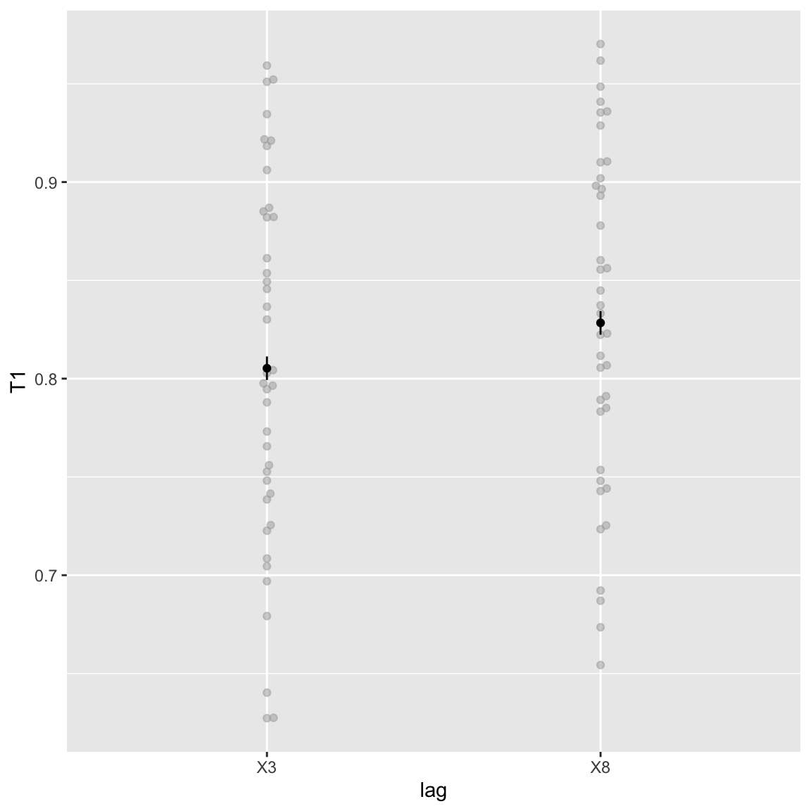

Study 2 - T1 main effect of Lag

Like T2|T1, T1 performance is also worse for the short lag (though only a little). Seems to be mostly driven by a few participants with relatively bad short-lag performance for T1. This effect was also reported in study 1.

Main effect of block

afex_plot(aov_study2_T1, x = "block", error = "within")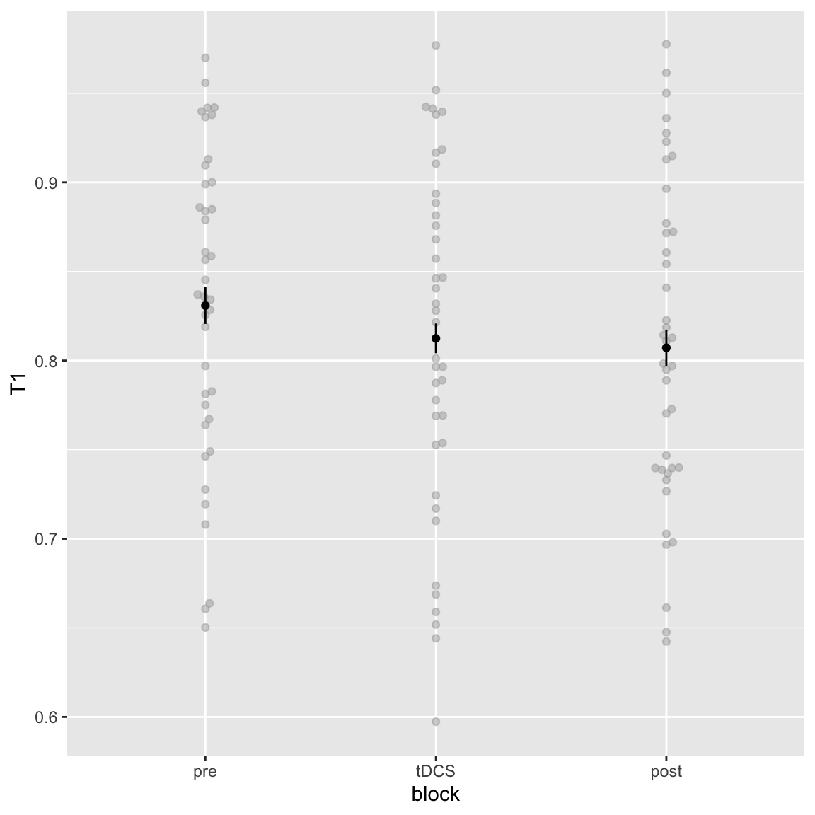

Study 2 - T1 main effect of Block

T1 performance seems to decrease slightly over the session. In study 1 this was also the case, for T1 and T2|T1, though here there was no effect of block on T2|T1.

Interaction: stimulation by session order

afex_plot(aov_study2_T1, x = "stimulation", trace = "session.order", error = "none")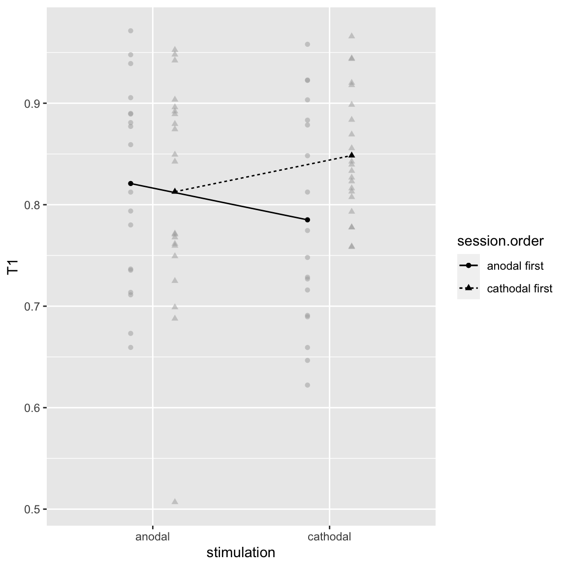

Study 2 - T1: Stimulation by Session Order

This interaction was also present for T2|T1 in both studies. There it seemed to reflect a learning effect, but here it goes in the opposite direction: T1 performance is worse in the 2nd session than the first…

Interaction: stimulation by session order by block

There is also a higher-order interaction with Block:

afex_plot(aov_study2_T1, x = "stimulation", trace =  "session.order", panel = "block", error = "none")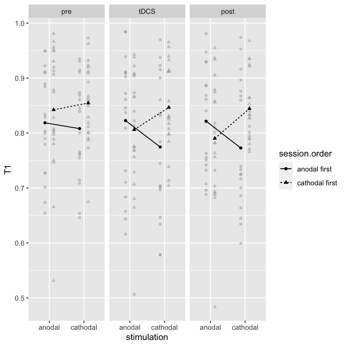

Study 2 - T1: Stimulation by Session Order by Block

The two-way interaction is strongest in the later two blocks. Again, this is the inverse of the learning effect, which was strongest in the first block.

London, R. E., & Slagter, H. A. (2021). No Effect of Transcranial Direct Current Stimulation over Left Dorsolateral Prefrontal Cortex on Temporal Attention. Journal of Cognitive Neuroscience, 33(4), 756–768. doi: 10.1162/jocn_a_01679 ↩︎

AB-tDCS

Group-level analyses

Leon Reteig

30 January, 2022

Setup environment

Load task data

Study 2

Study 1

Reformat

Group analysis

Line plots cf. London & Slagter (2021)

Study 1

Study 2

RM ANOVA

Study 1 - T2|T1

Main effect of lag

Main effect of block

Interaction: block by stimulation by lag

Interaction: stimulation by session order

Interaction: stimulation by session order by block

Study 2 - T2|T1

Main effect of lag

Interaction: block by stimulation by lag

Interaction: stimulation by session order

Interaction: stimulation by session order by lag

Interaction: stimulation by session order by lag by block

Study 2 - T1

Main effect of lag

Main effect of block

Interaction: stimulation by session order

Interaction: stimulation by session order by block