Spontaneous eye blink rate does not predict attentional blink size, nor the effects of tDCS on attentional blink size
Leon C. Reteig
1,2l.c.reteig@uva.nl
Lionel A. Newman
3K. Richard Ridderinkhof
1,2Heleen A. Slagter
1,4h.a.slagter@vu.nl
- Department of Psychology, University of Amsterdam
- Amsterdam Brain and Cognition, University of Amsterdam
- Department of Artificial Intelligence and Cognitive Engineering, University of Groningen
- Department of Applied and Experimental Psychology, Vrije Universiteit Amsterdam
Abstract
The attentional blink (AB) phenomenon illustrates our limited capacity to process incoming information. When tasked to identify two targets embedded in close temporal proximity in a stream of distractors, the second target is often missed. The magnitude of the AB (the proportion of times this second target is missed) varies considerably across individuals. Here, we examined two factors that might drive these individual differences: baseline dopamine levels and cortical excitability. We measured spontaneous Eye Blink Rate (sEBR) as a proxy for dopamine levels, and attempted to manipulate cortical excitability using transcranial Direct Current Stimulation (tDCS). Participants (n=40) performed an AB task before, during, and after anodal or cathodal tDCS to the left dorsolateral prefontal cortex, in two separate sessions. At the start of each session, we measured their sEBR. sEBR had good test-retest reliability across the sessions. Test-retest reliability for AB magnitude was moderate, but in line with previous reports. We found no linear- or U-shaped relationhip between sEBR and AB magnitude at baseline (before tDCS onset), with more evidence for the null hypothesis. Lastly, we also did not find an association between sEBR and the effect of tDCS on AB magnitude (neither anodal nor cathodal tDCS, compared to baseline). Larger-scale studies with more direct measures of dopamine and cortical excitability are called for to advance our understanding of their effects on the attentional blink, and rapid, selective gating of information, more generally.library(papaja) # APA formatted manuscripts
library(knitr) # rmarkdown output
library(tidyverse) # importing, transforming, and visualizing data frames
library(lubridate) # calculations with dates and time
library(psych) # intra-class correlations
library(broom) # transform model outputs into data frames
library(BayesFactor) # Bayesian correlations
library(cocor) # significance tests for difference between correlations
library(cowplot) # themes and placement of graphs (installed from github)
library(kableExtra) # complex tables
library(here) # (relative) file paths
source(here("src", "lib", "twolines.R")) # test for U-shaped correlations
# online: (http://webstimate.org/twolines/twolines.R)
source(here("src", "lib", "appendixCodeFunctionsJeffreys.R")) # replication Bayes factors
# online: https://osf.io/9d4ip/
knitr::opts_chunk$set(results='hide', message=FALSE, warning=FALSE)
base_font_size <- 9;
geom_text_size <- (base_font_size-1) * 0.35 # so geom_text size is same as axis text
base_font_family <- "Helvetica";# Seed for random number generation
set.seed(42)
knitr::opts_chunk$set(cache.extra = knitr::rand_seed)# data from these subjects should be discarded; they only did a single session
subs_incomplete <- c("S03", "S14", "S25", "S29", "S31", "S38", "S43", "S46") # read subject info
df_sub_info <- read_csv2(here("data","subject_info.csv"), col_types = cols(
subject = col_character(),
session = col_integer(),
polarity = col_character(),
time = col_datetime("%*%d.%m.%Y %H:%M"),
gender = col_character(),
age = col_integer(),
sleep_hours = col_double(),
sleep_quality = col_integer(),
alcohol_glasses = col_integer(),
smoker = col_character(),
caffeine_today = col_double(),
caffeine_usual = col_double(),
contacts_glasses = col_character(),
EEG_experience = col_character()
)) %>%
#filter out subs with incomplete data; and S42 (no data at all)
filter(!(subject %in% c(subs_incomplete,"S42"))) data_path <- here("data","AB") # top-level folder with task data
# list all the .txt files in folders of individual subjects
files <- dir(data_path, pattern = "*.txt", recursive = TRUE)# load single trial data
df <- data_frame(filename = files) %>% # store file list in column of data frame
mutate(file_contents = map(filename, # for each file, add table inside the .txt file
# make full path with file.path, pass to read_tsv
~read_tsv(file.path(data_path,.), col_types = cols( # parse column as:
totalTrial = col_integer(), # trial number from 1st trial
block = col_integer(), # block number
trial = col_integer(), # trial number this block
lag = col_integer(), # lag 3 or lag 8 trial
T1pos = col_integer(), # T1 position in stream
T1letter = col_character(), # actual green letter / T1
T1resp = col_character(), # which letter participant thought was green / T1
T2letter = col_character(), # actual red letter / T2
T2resp = col_character(), # which letter participant thought was red / T2
T1acc = col_integer(), # participant's T1 response was correct (1) or not (0)
T2acc = col_integer(), # participant's T2 response was correct (1) or not (0)
T1T2acc = col_integer() # code for T2 given T1 accuracy
))
)) %>%
unnest() # for each file, unfold the table in file_contents# clean single trial data
df_clean <- df %>%
# use file names to create separate columns for each subject/session/polarity/block ID
separate(filename, into = c("prefix","subject","ses_pol","block"), sep = "_") %>%
separate(ses_pol, into = c("session", "polarity"), 1) %>%
mutate(session = as.integer(session),
# remove numbers due to extra files, and file extension
block = str_replace_all(block, c("[0-9]" = "", ".txt" = "")),
# translate tDCS codes into "anodal" and cathodal
polarity = str_replace_all(polarity, c("B" = "anodal", "I" = "cathodal")),
# "D" means different things for S01--S21 then S22--S49
sub_id = as.integer(str_remove(subject,"S")), # get subject number without S
polarity = replace(polarity, sub_id <= 21 & polarity == "D", "cathodal"),
polarity = replace(polarity, sub_id > 21 & polarity == "D", "anodal")) %>%
select(-prefix,-sub_id) %>% # drop junk/ helper columns
filter(!(subject %in% subs_incomplete)) # discard data from single-session subjects# aggregate and compute summary measures
df_AB <- df_clean %>%
group_by(subject, session, block, polarity, lag) %>%
summarise(trials = n(),
T1 = sum(T1acc)/trials, # T1 accuracy
T2 = sum(T2acc)/trials, # T2 accuracy
T2_given_T1 = sum(T2acc[T1acc == 1])/sum(T1acc)) %>% # T1|T2 accuracy
ungroup()1 Introduction
We are constantly barraged by sensory information beyond our limited processing capacity. This is clearly brought to light by the attentional blink (AB) phenomenon: detection of the second of two targets (T2) is impaired for 100–500 ms after the initial target (T1) is presented within a stream of distractors (Raymond, Shapiro, and Arnell 1992; for reviews, see Dux and Marois 2009; Martens and Wyble 2010). Although the AB would seem to be a fundamental bottleneck, there are large individual differences in the magnitude of the AB (i.e., the proportion of times that T2 is missed vs. seen) (Willems and Martens 2016). Some participants nearly always miss T2, a small group of others do not have an AB at all (e.g. Martens et al. 2006), and most participants fall somewhere between these two extremes. The source of these individual differences remains largely unknown. Here, we examine two potential modulators of AB magnitude: baseline dopamine levels, and changes in cortical excitability induced by transcranial Direct Current Stimulation (tDCS).
London and Slagter (2015) were the first to study whether the effects of tDCS on the AB differ across individuals. tDCS can change the excitability of neurons from outside the skull, by passing a weak electrical current between an anodal and cathodal electrode (Gebodh et al. 2019). Anodal and cathodal tDCS are generally assumed to have opposite effects on cortical excitability. While this holds in non-human work (Purpura and McMurtry 1965; Bindman, Lippold, and Redfearn 1964) and the human motor cortex (Nitsche and Paulus 2000, 2001), it is likely an oversimplification (Liu et al. 2018) and might not generalize to other brain areas (Bestmann, De Berker, and Bonaiuto 2015; Parkin, Ekhtiari, and Walsh 2015). Nonetheless, London and Slagter (2015) found a differential effect of anodal vs. cathodal tDCS over the left dorsolateral prefrontal cortex (lDLPFC) at the individual subject level. Those individuals that showed a decrease in AB magnitude during anodal tDCS (compared to a baseline measurement) tended to show an increase during cathodal tDCS, and vice versa.
Many factors may influence the effect of tDCS on a given individual (Krause and Cohen Kadosh 2014; Li, Uehara, and Hanakawa 2015). One of the most prominent candidates is baseline cortical excitability, i.e. the balance of excitation and inhibition in the cortex (before tDCS onset). Krause, Márquez-Ruiz, and Cohen Kadosh (2013) suggested that the behavioral outcome of tDCS is governed by an Inverted-U-shaped relationship with cortical excitability. The effect of anodal/cathodal on a given individual would then depend on his or her position on this excitability axis (Figure 1.1, left panel). Individuals with excess excitation compared to the optimum would benefit from cathodal but not anodal tDCS, whereas over-inhibited inviduals would benefit from anodal but not cathodal tDCS. This matches the pattern of performance changes reported by London and Slagter (2015).
In the present study, we aimed to extend the findings of London and Slagter (2015) by examining the influence of dopamine. Dopaminergic projections are pervasive and shape global brain activity (Schultz 2007; Björklund and Dunnett 2007). In particular, dopaminergic signalling between the striatum and the prefrontal cortex is crucial for healthy cognitive functioning (Nieoullon 2002; Robbins and Arnsten 2009). Striatal dopamine has been linked to updating of goal representations and gating of information in the prefrontal cortex (Cohen, Aston-Jones, and Gilzenrat 2004; Cools and D’Esposito 2011)—processes that both seem to go awry in the AB. Indeed, several lines of evidence implicate dopamine in the AB. First, activity in the ventral striatum differentiates between trials in which T2 was seen or missed, both when measured with intracranial EEG (Slagter et al. 2017) and with fMRI (Slagter et al. 2010). Changing dopamine levels by administering L-DOPA can change the size of the AB in Parkinson patients (Slagter et al. 2016) (although dopamine antagonists in healthy individuals might not affect the AB (Gibbs et al. 2007)). Finally, AB size is correlated to dopamine receptor binding in the striatum as measured with Positron Emission Tomography (PET) (Slagter et al. 2012).
The relationship between dopamine and cognitive function appears to follow an Inverted-U shape, where both too high and too low levels of dopamine hurt performance (Cools and D’Esposito 2011). Slagter et al. (2012) proposed this also holds for the AB, which should be smallest at an optimal level of (striatal) dopamine. Too low levels of dopamine would restrict gating such that T2 is prevented from being processed; too high levels of dopamine would cause interference by “opening the gate too far” such that distractors are also processed. However, this model has not been formally tested, partly because it is so difficult to assess dopamine in humans without invasive measures such as PET.
There is converging evidence that spontaneous Eye Blink Rate (sEBR) could serve as such a non-invasive index of striatal dopamine (for a review, see Jongkees and Colzato 2016). One study indeed found a negative correlation between sEBR and the AB (Colzato et al. 2008), suggesting that inviduals with higher levels of dopamine have a smaller AB. However, a later study was unable to replicate this result (Slagter and Georgopoulou 2013).
No study to date has investigated the combined effects of dopamine and tDCS on the AB. But we do know that dopamine is an important moderator of the neurophysiological effects of tDCS (Stagg and Nitsche 2011). Dopaminergic activity is necessary for tDCS to have physiological after-effects, as these are abolished when dopamine receptors are blocked (Nitsche et al. 2006). Dopamine also shapes the time course and direction of tDCS-induced changes in cortical excitability: dopamine agonists may prolong the inhibitory effects of cathodal tDCS, and flip the anodal effect from excitatory to inhibitory (Kuo, Paulus, and Nitsche 2008).
Furthermore, two recent studies suggest that both tDCS and dopamine levels interact to determine cognitive performance in a systematic manner (Wiegand, Nieratschker, and Plewnia 2016). These capitalize on genetic differences in dopamine activity caused by a common polymorphism of the gene coding for the COMT enzyme. This enzyme regulates dopamine levels, especially in the prefrontal cortex (Käenmäki et al. 2010). Individuals that are homozygous for the Met-allele of the gene exhibit higher levels of cortical dopamine; individual homozygous for the Val-allele exhibit lower levels of dopamine (Schacht 2016). In one study, cathodal tDCS decreased performance on a go-no go task, but only in Val-homozygotes (Nieratschker et al. 2015); in the other study, anodal tDCS decreased performance on a different aspect of the task, and only in Met-homozygotes (Plewnia et al. 2013). Wiegand, Nieratschker, and Plewnia (2016) synthesized these findings in a model (Figure 1.1, right panel), proposing that individuals with low dopinamergic tone (e.g. Val-homozygotes) benefit from anodal but not cathodal tDCS, whereas individuals with high dopaminergic tone (e.g. Met-homozygotes) benefit from cathodal but not anodal tDCS. The outcome of anodal or cathodal tDCS would then differ as a function of baseline dopamine levels, which could provide another explanation for individual differences like those reported by London and Slagter (2015).
In the present study, we aimed to shed more light on the relation between dopamine and the AB, as well as the modulatory role that dopamine might play in the effects of tDCS on the AB. Following London and Slagter (2015), participants performed an AB task before, during, and after anodal or cathodal tDCS to the lDLPFC, in two separate sessions. At the start of each session, we measured sEBR as a proxy for baseline dopamine levels. First, we investigated whether sEBR is a reliable measure, as there is little data on the test-retest reliability of sEBR (Jongkees and Colzato 2016). Our study design with two sEBR-measurements per individual is uniquely suited to help fill this gap. Second, we examined how sEBR relates to AB magnitude. One study found a significant negative correlation (Colzato et al. 2008), but this was not replicated in a second study (Slagter and Georgopoulou 2013). Furthermore, both of these studies only tested for a linear relationship, although there is mounting evidence that the relationship between dopamine and cognitive performance is Inverted-U-shaped (Cools and D’Esposito 2011). Third, we assessed whether the effects of tDCS on AB magnitude depend on sEBR. Following the model in Figure 1.1 (Krause, Márquez-Ruiz, and Cohen Kadosh 2013; London and Slagter 2015; Wiegand, Nieratschker, and Plewnia 2016), anodal tDCS should increase performance (i.e., decrease AB magnitude) in low dopamine (i.e., low sEBR) individuals, but decrease performance in high dopamine individuals, and vice versa for cathodal tDCS.
knitr::include_graphics("figures/figure_1_model.png", auto_pdf = TRUE)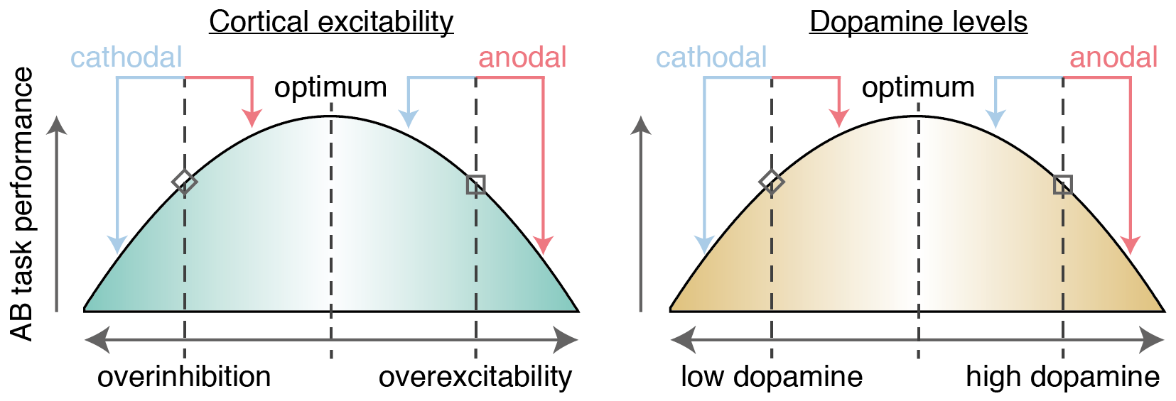
Figure 1.1: Model where AB task performance is dependent on cortical excitability (left, London and Slagter 2015) and dopamine levels (right, Wiegand, Nieratschker, and Plewnia 2016). Whether anodal (red arrows) or cathodal (blue arrows) tDCS improves performance depends on the baseline starting point on these axes, as shown in two example cases. First, an individual with relatively low levels of dopamine / cortical excitability (diamond shape) should benefit from anodal tDCS (as they move closer to the optimum), whereas cathodal tDCS would be detrimental (as they are pushed further away from the optimum). Reversely, an individual with high levels of dopamine / cortical excitability (square shape) would benefit from cathodal but not anodal tDCS.
2 Materials and methods
A different set of results based on this dataset were reported in (Reteig et al. 2019b). We include the full materials and methods here for convenience.1
2.1 Participants
sample_info <- df_sub_info %>%
  distinct(subject,gender,age) #only one row per subject
n_total <- nrow(sample_info)
n_female <- sum(sample_info$gender == "female")
age_mean <- mean(sample_info$age, na.rm = TRUE)
age_sd <- sqrt(sum((sample_info$age - age_mean)^2,
na.rm=TRUE)/sum(!is.na(sample_info$age))) # population SD
age_min <- min(sample_info$age, na.rm = TRUE)
age_max <- max(sample_info$age, na.rm = TRUE)
mean_T1 <- mean(df_AB$T1)Fourty-eight participants took part in total, 8 of whom were excluded after the first session. One participant was excluded excluded as a precaution because they developed an atypical headache after the first session, and we could not rule out this was related to the tDCS. Another stopped responding to our requests to schedule the second session. The remaining six participants were excluded because their mean T1 accuracy in the first session was too low, which would leave too few trials to analyze, because our T2 accuracy measure included only trials in which T1 was seen. We used a cut-off of 63% T1 accuracy as an exclusion criterium, which was two standard deviations below the mean of a separate pilot study (n = 10).
This left a final sample of 40 participants (29 female, mean age = 20.94, SD = 2.45, range = 18–28). This sample size was determined a priori to slightly exceed London and Slagter (2015) (n = 34). Mean T1 accuracy in the remaining 40 participants was 82%, which is comparable to previous studies using this task (86% in London and Slagter 2015; in 82% in Slagter and Georgopoulou 2013).
The experiment and recruitment took place at the University of Amsterdam. All procedures for this study were approved by the ethics review board of the Faculty for Social and Behavioral Sciences, and complied with relevant laws and institutional guidelines. All participants provided their written informed consent and were compensated with course credit or €10 per hour (typically €65 for completing two full sessions).
2.2 Procedure
# Session intervals in days
ds <- df_sub_info %>%
  select(subject,session,time) %>%
  spread(session,time, sep = "_") %>% # times for session_1 and session_2
  # count the number of integer days in the interval between sessions
  mutate(d_d = (session_1 %--% session_2) %/% days(1)) %>%
  count(d_d, sort = TRUE)
# determine session order
so <- df_sub_info %>%
count(session,polarity) %>%
filter(session == 1)The study procedures were identical to London and Slagter (2015): participants received anodal and cathodal tDCS in separate sessions (Figure 2.1), which typically took place exactly one week apart (for 29 participants; sessions were separated by 6 days for 6 participants; 8 days for 3 participants; 4 days for 1 participant; 10 days for 1 participant). The time in between served to keep the sessions as similar as possible, and to minimize the risk of tDCS carry-over effects. 18 participants received anodal tDCS in the first session and cathodal tDCS in the second, and vice versa for the remaining 22 participants.
First, participants experienced the sensations induced by tDCS in a brief trial stimulation (see the tDCS section). Next, sEBR was measured for 6 minutes (see the sEBR section), after which participants completed 20 practice trials of the task (see the Task section). For the main portion of the experiment, participants performed three blocks of the task (Figure 2.1): before tDCS (baseline), during anodal/cathodal tDCS (tDCS), and after tDCS (post).
Within each block of the task, participants took a self-timed break every 50 trials (~5 minutes); between the blocks, the experimenter walked in. Participants performed the task for exactly 20 minutes during the baseline and post blocks. During the tDCS block, the task started after the 1-minute ramp-up of the current was complete, and continued for 21 minutes (constant current, plus 1-minute of ramp-down).
knitr::include_graphics("figures/figure_2_procedure.png", auto_pdf = TRUE)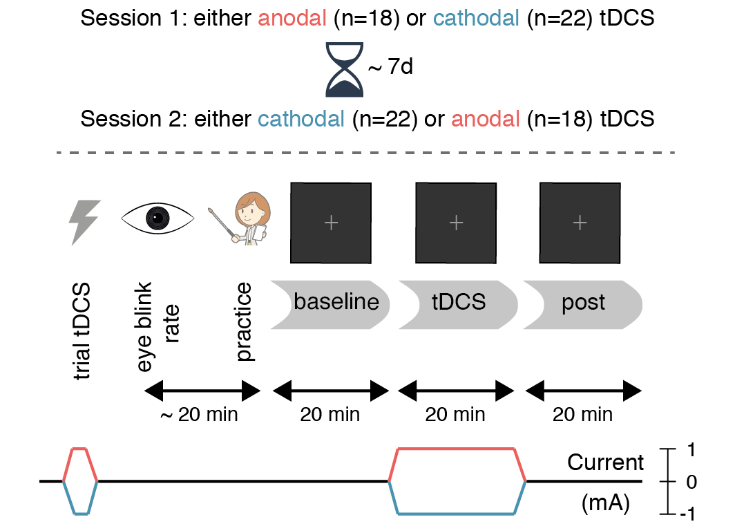
Figure 2.1: Experimental design. Spontaneous eye blink rate was measured for 6 minutes prior to the start of the task. Then (following a short practice block), participants performed three 20-minute blocks of the attentional blink task: a baseline block without stimulation, a tDCS block during 20 minutes of anodal (red) or cathodal (blue) stimulation, and finally a post-test block (also without stimulation). The second session (typically 7 days later at the same time of day) was identical, except that the tDCS polarity was reversed.
2.3 Task
The attentional blink task (Figure 2.2) was almost identical to the one used in London and Slagter (2015) and Slagter and Georgopoulou (2013), which in turn was based on a task designed by Dux and Marois (2008). A rapid serial visual presentation stream of 15 letters (cf. 17 letters in London and Slagter (2015)) was shown on each trial, using Presentation software (Neurobehavioral Systems, Inc.). Each letter was displayed for 91.7 ms (11 frames at 120 Hz) on a dark gray background. The letters were presented in font size 40 (font: Courier New) at a viewing distance of 90 cm. On each trial, the letters were randomly sampled without replacement from the alphabet, excluding the letters I, L, O, Q, U and V, as they were too similar to each other. All distractor letters were mid-gray, whereas T1 and T2 were colored. T1 was red and always appeared at position 5 in the stream. T2 was green and followed T1 after either 2 distractors (lag 3) or 7 distractors (lag 8) (cf. lags 2, 4 and 10 in London and Slagter (2015)).
The letter stream was preceded by a fixation cross (same color as the letters) presented for 1750 ms and followed by another fixation cross (presented for 1000 ms). Finally, the participant was prompted to type in (using a standard keyboard) the letter they thought was presented as T1 (“Which letter was red?”), followed by T2 (“Which letter was green?”).
trial_counts <- df_AB %>%
  group_by(lag) %>%
  summarise_at(vars(trials), funs(mean, min, max, sd))
Trial duration varied slightly because both the T1 and T2 response questions were self-paced, so some participants completed more trials than others depending on their response times. On average, participants completed 130 short lag trials (SD = 17; range = 78–163) and 65 long lag trials (SD = 9; range = 39–87) per 20-minute block.
knitr::include_graphics("figures/figure_3_task.png", auto_pdf = TRUE)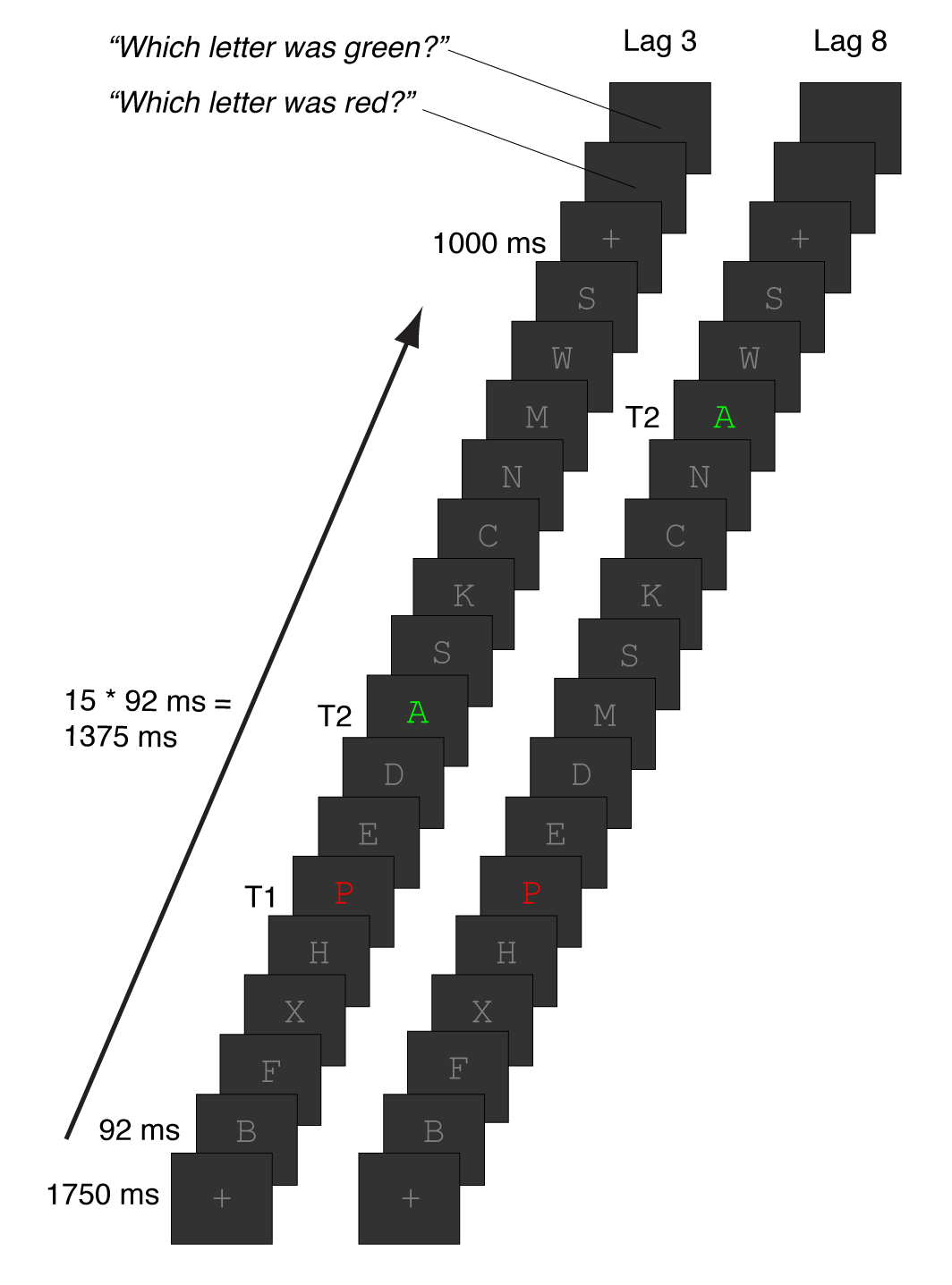
Figure 2.2: Attentional blink task. Participants viewed rapid serial visual presentation streams of 15 letters, all of which were distractors (gray letters) except for T1 and T2. T1 was presented in red at position 5; T2 was presented in green and followed T1 after 2 distractors (lag 3, inside the AB window) or 7 distractors (lag 8, outside the AB window). At the end of the trial, participants reported the identity of T1 and then T2 (self-paced).
2.4 tDCS
Transcranial direct current stimulation was delivered online (i.e. during performance of the attentional blink task) using a DC-STIMULATOR PLUS (NeuroCare Group GmbH). The current was ramped up to 1 mA in 1 minute, stayed at 1 mA for 20 minutes, and was ramped down again in 1 minute.
One electrode was placed at F3 (international 10-20 system) to target the lDLPFC; the other was placed over the right forehead, centered above the eye (approximately corresponding to position Fp2). Both electrodes were 5 x 7 cm in size (35 cm2), leading to a current density of 0.029 mA/cm2. The electrode montage and tDCS parameters are identical to London and Slagter (2015), with two exceptions. First, we also measured EEG (see the sEBR section), so the EEG electrodes and headcap were applied on top of the tDCS electrodes. Second, we used Ten20 paste (Weaver and Company) as the conductive medium, whereas London and Slagter (2015) used sponges soaked in saline.
Participants received either anodal tDCS (anode on F3, cathode on right forehead) or cathodal tDCS (cathode on F3, anode on right forehead) in separate sessions. The procedure was double-blinded: both the participant and the experimenters were unaware which polarity was applied in a given session. The experimenter loaded a stimulation setting on the tDCS device (programmed by someone not involved in data collection), without knowing whether it was mapped to anodal or cathodal tDCS. In the 2nd session, the experimenter loaded a second setting mapped to the opposite polarity (half the dataset), or simply connected the terminals of the device to the electrodes in the opposite way.
At the start of the experiment, participants received a brief trial stimulation, based on which they decided whether or not they wanted to continue with the rest of the session. The experimenter offered to terminate the experiment in case tDCS was experienced as too uncomfortable, but none of the participants opted to do so. For the trial stimulation, the current was ramped up to 1 mA in 45 seconds, stayed at 1 mA for 15 seconds, and was ramped down again in 45 seconds.
2.5 sEBR
Movement of the eyelids across the eyes affects the electrical potential that naturally exists across the eyeball (Matsuo, Peters, and Reilly 1975). Blinks can thus be recorded with electrodes placed on the face and/or scalp (Luck 2005).
We used a BioSemi ActiveTwo system with 64 Ag/AgCl active electrodes, placed according to the (10-10 subdivision of the) international 10-20 system. Two pairs of additional external electrodes were placed to record the electro-oculogram (EOG): above and below the left eye, and next to the left and right outer canthi. Finally, another pair of electrodes on the left and right earlobes served as the reference. This full setup was used because we also recorded the EEG during task performance. This dataset is available elsewhere (Reteig et al. 2019a).
# Session intervals in hours
hs <- df_sub_info %>%
  select(subject,session,time) %>%
  spread(session,time, sep = "_") %>% # times for session_1 and session_2
  # pull the hour of day and subtract
  mutate(d_h = abs(hour(session_2) - hour(session_1))) %>%
  count(d_h, sort = TRUE)
sEBR was recorded for 6 minutes after setting up the EEG in each session. Participants were asked to sit still and look straight ahead at a white wall (about 1 meter away). Participants were told they were allowed to move their eyes, but the experimenter made no mention of eye blinks. The “cover story” was that we needed to monitor the quality of the EEG signal before being able to start the recordings. Because blink rate can increase in the evening (Barbato et al. 2000), but is stable during the day time (Barbato et al. 2000; Doughty and Naase 2006), we made sure all recordings were completed before 5 PM. Most participants started their first and second sessions at the exact same time of day (34 participants; 4 participants started their second session 5 hours earlier/later than their first, 2 started 3 hours earlier/later).
The raw data were preprocessed using the EEGLAB toolbox (Delorme and Makeig 2004) in MATLAB (MathWorks, Inc.). First, data were re-referenced offline to the average of the earlobe electrodes. Next, horizontal and vertical EOG channels were created by subtracting the signals from each member of a horizontal/vertical electrode pair. A high-pass filter with a cut-off of .5 Hz was then applied. Finally, we ran an independent component analysis (ICA) to capture the eye blink events in a single time series. For each recording, we visually inspected the independent components and selected one that appeared to contain the eye blink signals, based on the waveform (large amplitude, positive deflections) and scalp distribution of the ICA weights (loading on frontal and EOG electrodes).
Eye blinks in this component were then detected using a semi-automatic procedure (cf. Slagter and Georgopoulou 2013; Kruis et al. 2016). First, a voltage threshold was set (initialized to the standard deviation of the signal) which captured most eye blink peaks. This threshold was moved up or down by the analyst if necessary. The sample with the maximum voltage between two threshold crossings was marked as an eye blink, with the restriction that two eye blinks must be at least 400 ms apart. We picked 400 ms as an upper estimate of the duration of a single blink (Caffier, Erdmann, and Ullsperger 2003). The analyst then inspected the output, and removed or added eye blinks in the case of clear false positives (e.g., a muscle contraction) or false negatives (e.g., an eye blink waveform did not exceed the threshold, or was followed by another clear eye blink within 400 ms).
2.6 Statistical analysis
# make text for general r-citations;
# withold certain packages to cite individually
r_citations <- cite_r(file = "r-references.bib",
                      pkgs = c("broom","cowplot","here","tidyverse","papaja","knitr","lubridate"),
                      withhold = FALSE,
                      footnote = TRUE)
Data were analyzed using R (Version 3.5.1; R Core Team 2018)2 from within RStudio (Version 1.1.463; RStudio Team 2016). Our analyses were focused on three depedendent variables. sEBR was expressed as the number of eye blinks per minute. For the AB, we examined T2|T1 accuracy, i.e. the percentage of trials where T2 was reported correctly, out of the subset of trials in which T1 was reported correctly. The size of the attentional blink (AB magnitude) was quantified by subtracting T2|T1 accuracy at lag 3 from T2|T1 accuracy at lag 8, for each session in each block. Lastly, we created AB magnitude change scores for each session by subtracting AB magnitude in the “baseline” block from the “tDCS” and the “post” blocks, respectively.
2.6.1 Reliability
We evaluated the test-retest reliability of sEBR and AB magnitude across sessions by computing intraclass correlations (ICCs) using the psych package (Version 1.8.10; Revelle 2018). We primarily report the single-rating, two-way ICC for absolute agreement, also known as ICC(2,1) in the conventions from Shrout and Fleiss (1979). This is the most appropriate ICC for test-retest reliability (Koo and Li 2016). In addition, we report Pearson’s correlation, to be able to compare the reliability of sEBR with Dang et al. (2017), and ICC(3,2), also known as Cronbach’s alpha (McGraw and Wong 1996), to compare our results with Kruis et al. (2016). We used the interpretation scheme in Koo and Li (2016), which classifies reliability as “poor” for ICCs < .5, .5 < ICC < .75 as “moderate”, .75 < ICC < .9 as “good”, and ICCs > .9 as “excellent”. For AB magnitude, we also report Pearson’s correlation, as this measure was used by all previous studies on the reliability of the AB (e.g. Dale, Dux, and Arnell 2013). Here we also used data from the baseline block only, to rule out any influence of tDCS on the reliability scores.
2.6.2 Relation between sEBR and baseline AB magnitude
2.6.2.1 Linear relationships
We calculated Pearson correlations to test for linear relationships between sEBR and AB magnitude. We also computed a Bayes factor for these correlations, as proposed by Ly, Verhagen, and Wagenmakers (2016) and implemented in the BayesFactor package (Version 0.9.12-4.2; Morey and Rouder 2018), with the standard prior distribution (\(\kappa\) = .33). This Bayes factor (\(BF_{01}\)) expresses the relative evidence for the null hypothesis of zero correlation, vs. the alternative hypothesis that there is a non-zero correlation. We use the interpretation scheme from Wagenmakers et al. (2018), where \(1 < BF_{01} < 3\) consitutes “anecdotal” evidence for the null, \(3 < BF_{01} < 10\) ~ “moderate” evidence, and \(10 < BF_{01} < 30\) ~ “strong” evidence.
Because Colzato et al. (2008) previously reported a negative relationship between sEBR and AB magnitude, we computed two additional Bayes Factors that incorporate this prior information. First, we used the same prior but folded all of its mass to negative effect sizes only, effectively providing a Bayes factor for a one-sided test (Wagenmakers, Verhagen, and Ly 2016). This Bayes factor (\(BF_{0-}\)) expresses the relative evidence for the null hypothesis of zero correlation, vs. the alternative hypothesis that there is a negative correlation. Second, we computed a replication Bayes Factor, by using the posterior from Colzato et al. (2008) as a prior (Verhagen and Wagenmakers 2014; Wagenmakers, Verhagen, and Ly 2016). This Bayes factor (\(BF_{0r}\)) expresses the relative evidence for the null hypothesis of zero correlation, vs. the alternative hypothesis that the correlation isas in Colzato et al. (2008).
2.6.2.2 Inverted-U-shaped relationships
To evaluate the presence of an (Inverted-) U-shaped relationship between sEBR and AB magnitude, we used the “two-lines test” as proposed by Simonsohn (2018). This test revolves around the core assumption in any U-shaped relationship: that a sign flip occurs at a break point in the data. Values on one side of this break point should exhibit a positive relationship (rising flank of the U); values on the other side should exhibit a negative relationship (falling flank of the U). The “two-lines test” first estimates the value of the break point based on a cubic spline fit to all of the data, and then computes two linear regressions to estimate the slopes on either side of the break point. Both slopes have to be significant and of opposite sign to reject the null hypothesis that there is no U-shaped relationship.
2.6.3 Relation between sEBR and the effect of tDCS on AB magnitude
We also calculated Pearson and Bayesian correlations between sEBR and AB magnitude change scores, cf. the relation between sEBR and AB magnitude at baseline. In general, such a correlation \(r_{A(Y-X)}\) between a change score \(Y-X\) (here, AB magnitude in the tDCS or post block minus the baseline score) and another variable \(A\) (here, sEBR), is a function of four components: 1) \(r_{AX}\): the correlation between \(A\) and the pre-test \(X\), 2) \(r_{AY}\): the correlation between \(A\) and the post-test \(Y\), 3) \(r_{XY}\): the correlation between pre- and post-test (i.e., the reliability), and 4) \(SD_y / SD_x\): the ratio between the standard deviations of the pre- and post-test (Gardner and Neufeld 1987; Griffin, Murray, and Gonzalez 1999). Next to the correlation with the difference score, we also computed these constituent components (reported in Tables 3.1 and 3.2). A complementary way to test for \(r_{A(Y-X)}\) is to test whether \(r_X\) and \(r_Y\) are significantly different. We used the Pearson-Filon test (1898) for this purpose, as implemented in the cocor package (Version 1.1-3; Diedenhofen and Musch 2015).
2.7 Data, materials, and code availability
All of the data, materials, and code for this study are available on the Open Science Framework3. The raw task data and sEBR recordings can be downloaded from this page [FIXME: Insert data citation]. The code to preprocess the sEBR data and perform the semi-automatic eye blink detection (cf. Slagter and Georgopoulou 2013; Kruis et al. 2016) is supplied in MATLAB scripts. We provide the statistical analysis code in the form of an R notebook, detailing all the analyses that we ran for this project, along with the results. We also include an Rmarkdown (Xie, Allaire, and Grolemund 2018) source file for this paper that can be run to reproduce the pdf version of the text, along with all the figures and statistics.
3 Results
# compute AB magnitude
df_ABmag <- df_AB %>%
  group_by(subject, session, polarity, block) %>% # for each unique factor combination
  summarise(AB_magnitude = last(T2_given_T1) - first(T2_given_T1)) %>% # subtract lags to replace data
  ungroup()
# create sEBR data frame
df_sEBR <- read_csv(here("data","sEBR","sEBR.csv"), col_types = cols(
subject = col_character(),
session = col_integer(),
tDCS_code = col_character(),
sEBR = col_double()
)) %>%
rename(polarity = tDCS_code) %>%
mutate(polarity = str_replace_all(polarity, c("B" = "anodal", "I" = "cathodal")),
# "D" means different things for S01--S21 then S22--S49
sub_id = as.integer(str_remove(subject,"S")), # get subject number without S
polarity = replace(polarity, sub_id <= 21 & polarity == "D", "cathodal"),
polarity = replace(polarity, sub_id > 21 & polarity == "D", "anodal")) %>%
select(-sub_id) %>%
filter(!(subject %in% subs_incomplete)) # discard data from single-session subjects3.1 Reliability
# Intra-class correlation for AB magnitude
ICC_ABmag <- df_ABmag %>%
  filter(block == "pre") %>%
  select(subject, session, AB_magnitude) %>%
  spread(session, AB_magnitude, sep = "_") %>% # create 2 sEBR columns: session 1 and session 2
  select(-subject) %>% # drop subjects column
  ICC(lmer=FALSE) # intra-class correlation
# Intra-class correlation for sEBR
ICC_sEBR <- df_sEBR %>%
select(subject, session, sEBR) %>%
spread(session, sEBR, sep = "_") %>% # create 2 sEBR columns: session 1 and session 2
select(-subject) %>% # drop subjects column
ICC(lmer=FALSE) # intra-class correlation, using AOV instead of LMER (no missing data)pearson_ABmag <- df_ABmag %>%
filter(block == "pre") %>%
select(subject, session, AB_magnitude) %>%
spread(session, AB_magnitude, sep = "_") %>%
cor.test(data = ., .$session_1, .$session_2,
method = "pearson", alternative = "two.sided")pearson_sEBR <- df_sEBR %>%
select(subject, session, sEBR) %>%
spread(session, sEBR, sep = "_") %>% # create 2 sEBR columns: session 1 and session 2
cor.test(data = ., .$session_1, .$session_2,
method = "pearson", alternative = "two.sided")# Plot AB over sessions
df_mean_AB <- df_AB %>%
group_by(session = factor(session), lag = factor(lag)) %>%
summarise(M = mean(T2_given_T1))
plot_lag3 <- df_AB %>%
left_join(df_ABmag) %>%
select(-T1,-T2,-trials) %>%
filter(block == "pre") %>%
spread(lag, T2_given_T1, sep = "_") %>%
mutate(session = factor(session),
subject = fct_reorder(subject, AB_magnitude)) %>%
ggplot(aes(subject,lag_8)) +
#coord_flip() +
geom_hline(data = df_mean_AB, aes(yintercept = M, colour = lag, linetype = session)) +
geom_linerange(aes(x = subject, group = subject, ymin = lag_3, ymax = lag_8, linetype = session),
color = "grey", show.legend = FALSE, position = position_dodge2(.75)) +
geom_point(shape = 21, aes(x = subject, y = lag_3), fill = "#E69F00",
colour = "white", stroke = 1, position = position_dodge2(.75)) +
geom_point(shape = 21, aes(x = subject, y = lag_8), fill = "#D55E00",
colour = "white", stroke = 1, position = position_dodge2(.75)) +
#geom_text(aes(label = round(AB_magnitude,2), x = T2_given_T1), size = 2) +
theme_minimal_hgrid(font_size = base_font_size, font_family = base_font_family) +
theme(axis.text.x=element_blank(), axis.ticks.x = element_blank(), axis.line.x = element_blank()) +
xlab("participant") +
scale_y_continuous("accuracy (T2|T1)", labels = scales::percent_format()) +
scale_colour_manual(values = c("#E69F00", "#D55E00")) +
NULL# function for test-retest plots
paired_plot <- function(df, lims, break_int, labs = waiver()) {
df_axes <- data.frame(
x = c(lims[1], -Inf),
xend = c(lims[2], -Inf),
y = c(-Inf, lims[1]),
yend = c(-Inf, lims[2])
)
ggplot(df, aes(session_1,session_2)) +
geom_abline(color = "grey") +
geom_point(shape = 21, fill = "gray25", size = 2, color = "white", stroke = .3) +
geom_segment(
data = df_axes,
aes(x = x, xend = xend, y = y, yend = yend),
size = 0.5,
inherit.aes = FALSE
) +
scale_x_continuous(breaks = seq(lims[1],lims[2],break_int),
labels = labs,
expand = expand_scale(mult = c(.1, .05))) +
scale_y_continuous(breaks = seq(lims[1],lims[2],break_int),
labels = labs,
expand = expand_scale(mult = c(.1, .05))) +
coord_fixed(clip ="off") +
theme_half_open(font_size = base_font_size, font_family = base_font_family) +
theme(axis.line = element_blank()) +
NULL
}# plot AB test-retest
ICC_label_ABmag = paste0("ICC(2,1) = ",
printnum(ICC_ABmag$results["Single_random_raters","ICC"], gt1 = F),
",\n",
"95% CI[",
printnum(ICC_ABmag$results["Single_random_raters","lower bound"], gt1 = F),
",",
printnum(ICC_ABmag$results["Single_random_raters","upper bound"], gt1 = F)
,"]")
plot_AB <- df_ABmag %>%
filter(block == "pre") %>%
select(subject, session, AB_magnitude) %>%
spread(session, AB_magnitude, sep = "_") %>%
paired_plot(c(.1,.7),.1, scales::percent_format(accuracy = 1)) +
annotate("text", label = ICC_label_ABmag, size = geom_text_size,
x = .1, y = .6, hjust = "left", vjust = "center") +
labs(title = "Attentional Blink magnitude", x = "session 1", y = "session 2") +
NULLWe first examined task performance in the baseline block of both sessions, i.e. before tDCS onset. All participants showed the characteristic AB effect in both sessions: T2|T1 accuracy was higher for lag 8 trials than for lag 3 (Figure 3.1A).
There was also a significant difference in AB magnitude (lag 8 minus lag 3 T2|T1 accuracy) between the sessions: (F(1, 39) = 16.53, p < .001). For most participants, AB magnitude was smaller in the 2nd session than the first (Figure 3.1B). The average difference in AB magnitude over sessions seemed to be driven by lag 3 performance only (Figure 3.1A), meaning the AB genuinely decreased with practice.
To be able to uncover relationships between sEBR and AB magnitude (see the subsequent sections), it is crucial that the test-retest reliability of both measures is adequate, i.e. that there is substantial agreement between the scores in session 1 and 2.
The intraclass correlation for AB magnitude (Figure 3.1B) is .60, indicating “moderate” test-retest reliability (Koo and Li 2016), with a 95% confidence interval of .25 (poor) – .79 (good). The standard (interclass) Pearson correlation for AB magnitude between sessions is comparable (r(38) = .68, CI95% [.47, .82]) and comparable to previous reports (Dale, Dux, and Arnell 2013).
# plot sEBR test-retest
ICC_label_sEBR = paste0("ICC(2,1) = ",
                        printnum(ICC_sEBR$results["Single_random_raters","ICC"], gt1 = F),
                        ",\n",
                        "95% CI[",
                        printnum(ICC_sEBR$results["Single_random_raters","lower bound"], gt1 = F),
                        ",",
                        printnum(ICC_sEBR$results["Single_random_raters","upper bound"], gt1 = F),
                        "]")

plot_sEBR <- df_sEBR %>%
  select(subject, session, sEBR) %>%
  spread(session, sEBR, sep = "_") %>%

  paired_plot(c(0,60),10) +
  annotate("text", label = ICC_label_sEBR, size = geom_text_size,
           x = 0, y = 50, hjust = "left", vjust = "center") +
  labs(title = "spontaneous Eye Blink Rate",
       x = "session 1",
       y = "session 2")
# combine plots
fig_retest_bottom <- plot_grid(plot_AB, plot_sEBR, labels = c("B","C"), align = 'h')
fig_retest <- plot_grid(plot_lag3, fig_retest_bottom, labels = c("A",""),
ncol = 1, rel_heights = c(1, 1.33))
fig_retest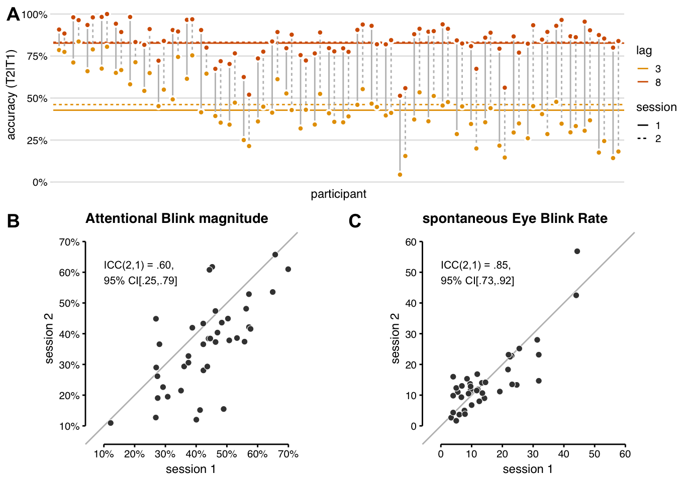
Figure 3.1: Reliability of the attentional blink and spontaneous eye blink rate. (A) All participants showed an attentional blink in both sessions: higher T2|T1 accuracy (% T2 correct in trials where T1 was also correct) for lag 8 (orange) than lag 3 (yellow). Horizontal lines show group-average T2|T1 accuracy. The attentional blink magnitude (lag 8 - lag 3) is slightly smaller in the 2nd session (dotted lines) than the first session (solid lines), due to better lag 3 performance on average. (B) AB magnitude for each participant in session 1 vs. 2. The intraclass correlation indicates moderate test-retest reliability, though the 95% confidence interval ranges all the way from poor to good. AB magnitude in (A) and (B) was calculated on the baseline block only, before tDCS onset. (C) sEBR values for each participant in session 1 vs. 2. The intraclass correlation indicates that the test-retest reliability for sEBR is good.
sEBR_EEG <- df_sEBR %>%
  left_join(df_sub_info, by = c("subject", "session", "polarity")) %>%
  group_by(EEG_experience,session) %>%
  summarise(n = n_distinct(subject), median_sEBR = median(sEBR))

median_sEBR2 <- median(df_sEBR$sEBR[df_sEBR$session == 2])
median_sEBR1 <- median(df_sEBR$sEBR[df_sEBR$session == 1])
sEBR_S27 <- df_sEBR$sEBR[df_sEBR$subject == "S27" & df_sEBR$session == 2]
sEBR_S27_diff <- diff(df_sEBR$sEBR[df_sEBR$subject == "S27"])

median_sEBR1_EEG <- sEBR_EEG$median_sEBR[sEBR_EEG$EEG_experience == "yes" & sEBR_EEG$session == 1]
median_sEBR2_EEG <- sEBR_EEG$median_sEBR[sEBR_EEG$EEG_experience == "yes" & sEBR_EEG$session == 2]
n_EEG <- sum(df_sub_info$EEG_experience == "yes" & df_sub_info$session == 1)
n_smoker <- sum(df_sub_info$smoker == "yes" & df_sub_info$session == 1)
n_contacts <- sum(df_sub_info$contacts_glasses == "contacts" & df_sub_info$session == 1)
In contrast to AB magnitude, sEBR (Figure 3.1C), did not differ significantly between sessions (F(1, 39) = 0.149, p = 0.701). We had some concerns that participants would blink less in the 2nd session, because they had been instructed (after the sEBR measurement in session 1) that blinking can cause artifacts in the EEG signal (recorded during task performance). Yet, if anything, median sEBR was slightly higher in the 2nd session (12.6) than the first (11.7). However, we also asked participants whether they had been in an EEG experiment before. Participants that had done so exhibited a greatly reduced median sEBR in both sessions (6.3 in session 1; 4.1 in session 2). Because these were only 6 cases in an already small sample, we are unsure whether this finding is robust, but it is a cautionary note to others aiming to measure sEBR using (a full setup of) EEG electrodes. Because smoking has been reported to increase sEBR (Klein, Andresen, and Thom 1993), we also asked whether participants self-identified as a smoker (n = 5). These individuals were not clear outliers in the distribution, neither were those wearing contact lenses (n = 4), which also generally should increase blink rate.
Most importantly, the test-retest reliability for sEBR was “good” (Koo and Li 2016), indicated by an intraclass correlation of .85 CI95% [.73, .92]. The Pearson correlation was r(38) = .84, CI95% [.72, .91] (cf. Dang et al. 2017); Cronbach’s alpha was .91 CI95% [.84, .95] (cf. Kruis et al. 2016).
One participant’s sEBR in session 2 seems remarkably high (57 blinks per minute), and is quite a bit higher in session 2 than in session 1 (difference of 12). However, we confirmed this was not a data quality issue, and rerunning the analyses without this participant did not qualitatively change the results in the subsequent sections. Hence, this participant was included in all analyses.
3.2 Relation between sEBR and baseline AB magnitude
lCorr_AB <- df_sEBR %>%
  left_join(df_ABmag) %>%
  filter(block == "pre") %>% # only baseline block
  nest(-session) %>% # for each session
  mutate(stats = map(data, ~cor.test(.$sEBR, .$AB_magnitude,
                                     alternative = "two.sided",
                                     method = "pearson"))) %>% # correlate sEBR to AB magnitude
  unnest(map(stats,tidy), .drop = TRUE) # make output into data frame, drop rest
uCorr_pre_session1 <- df_sEBR %>%
left_join(df_ABmag) %>%
filter(block == "pre", session == 1) %>%
twolines(AB_magnitude~sEBR, graph = 1, data = .)uCorr_pre_session2 <- df_sEBR %>%
left_join(df_ABmag) %>%
filter(block == "pre", session == 2) %>%
twolines(AB_magnitude~sEBR, graph = 1, data = .)# Make df with all results of model fits
x_1 <- pull(filter(df_sEBR, session == 1),sEBR)
x_2 <- pull(filter(df_sEBR, session == 2),sEBR)
df_u <- bind_cols(tribble(
~session, ~breakpoint, ~b_1, ~b_2,
"session 1", uCorr_pre_session1$xc, uCorr_pre_session1$b1, uCorr_pre_session1$b2,
"session 2", uCorr_pre_session2$xc, uCorr_pre_session2$b1, uCorr_pre_session2$b2,
), tribble(
~intercept, ~d,
uCorr_pre_session1$glm1$coefficients[1], uCorr_pre_session1$glm1$coefficients[4],
uCorr_pre_session2$glm1$coefficients[1], uCorr_pre_session2$glm1$coefficients[4],
), tribble(
~fit, ~x, ~xmin, ~xmax,
uCorr_pre_session1$yhat.smooth[order(x_1)], x_1[order(x_1)], min(x_1), max(x_1),
uCorr_pre_session2$yhat.smooth[order(x_2)], x_2[order(x_2)], min(x_2), max(x_2)
))Based on the results of Colzato et al. (2008), we should expect to find a negative correlation between sEBR and AB magnitude (in the baseline block). However, the correlation here was not significant in either session 1 (r(38) = .08, CI95% [-.24, .38], p = .637), or session 2 (r(38) = .003, CI95% [-.31, .31], p = .987). The direction of the effect is close to zero or slightly positive (Figure 3.2), which is not in accord with Colzato et al. (2008).
BF_default <- df_sEBR %>%
  left_join(df_ABmag) %>%
  filter(block == "pre") %>% # only baseline block
  nest(-session) %>% # for each session
  mutate(BF_null = 1 / map_dbl(data, ~extractBF(correlationBF(.$sEBR, .$AB_magnitude),
                     onlybf = TRUE))) # correlate sEBR to AB magnitude
BF_one_sided <- df_sEBR %>%
left_join(df_ABmag) %>%
filter(block == "pre") %>% # only baseline block
nest(-session) %>% # for each session
mutate(BF_one_sided = map(data, ~rownames_to_column(extractBF(
correlationBF(.$sEBR, .$AB_magnitude, nullInterval = c(-1,0)))))) %>% # correlate sEBR to AB magnitude
unnest(BF_one_sided, .drop = T) %>%
mutate(BF_null = 1/ bf) %>% # transform to evidence for null
filter(!str_detect(rowname, "!")) # filter out complement to intervalbf0R_1 <- 1 / repBfR0(nOri = 20, rOri = -.530, nRep = lCorr_AB$parameter[1]+2, rRep = lCorr_AB$estimate[1])
bf0R_2 <- 1 / repBfR0(nOri = 20, rOri = -.530, nRep = lCorr_AB$parameter[2]+2, rRep = lCorr_AB$estimate[2])Bayesian correlations show that the data are BF01 = 2.57 times (session 1) and BF01 = 2.84 times (session 2) more likely under the null hypothesis, using the default prior. This constitutes some evidence for absence of a correlation, though not more than anecdotal. If we evaluate the prior over negative effect sizes only (based on the negative correlation in Colzato et al. 2008), the support for the null increases slightly and becomes moderate (session 1: BF0- = 3.90, session 2: BF0- = 2.87). Finally, if we use the correlation as in Colzato et al. (2008) (r(18) = -.53) as a prior (Wagenmakers, Verhagen, and Ly 2016), the support for the null hypothesis becomes strong (session 1: BF0r = 15.80, session 2: BF0r = 10.43).
We also probed for an Inverted-U-shaped relationship between sEBR and AB magnitude, using the “two lines test” (Simonsohn 2018). In session 1, a cubic spline-fit indeed suggests an Inverted-U-shaped relationship (Figure 3.2). The linear regressions do as well, since the first slope is positive (b = .012, p = .058) and the second is negative (b = -.006, p = .602). However, neither slope is significant. Furthermore, this pattern is absent in session 2 (line 1: b = .001, p = .931; line 2: b = .003, p = .545), with the spline fit also showing a more erratic pattern.
df_sEBR %>%
  left_join(df_ABmag) %>%
  mutate(session = paste("session", session)) %>% # add "session" to facet labels
  left_join(select(df_u, session, breakpoint)) %>% # add breakpoint info
  filter(block == "pre") %>% # AB mag from baseline only
  mutate(reg = factor(ifelse(sEBR <  breakpoint, 1, 2))) %>% # colors based on breakpoint

  ggplot(aes(sEBR, AB_magnitude)) +
  facet_wrap(~session, ncol = 1) + # for each session
  geom_segment(data = unnest(df_u), # plot the first linear fit
               aes(x = xmin, xend = breakpoint,
                   y = intercept + b_1*(xmin - breakpoint), # solve interrupted regression
                   yend = intercept),
               colour = "#009E73") +
  geom_segment(data = unnest(df_u), # plot the 2nd linear fit
               aes(x = breakpoint, xend = xmax,
                   y = intercept + d,
                   yend = intercept + b_2*(xmax - breakpoint) + d),  # solve for ending-y
               colour = "#CC79A7") +
  geom_smooth(method = "lm", se = FALSE, colour = "gray50") + # plot the overall linear fit
  geom_point(shape = 21, fill = "gray25", size = 2, aes(colour = reg), stroke = .3, show.legend = FALSE) +
  geom_path(data = unnest(df_u), aes(x = x, y = fit), # plot the spline fit
            lty = "dashed", colour = "gray50", size = 1) +
  scale_x_continuous("spontaneous Eye Blink Rate (per min)", limits = c(0,60),
                     breaks = seq(0,60,10), expand = c(0,0)) +
  scale_y_continuous("Attentional blink magnitude", limits = c(.1,.7),
                     breaks = seq(.1,.7,.1), labels = scales::percent_format(accuracy = 1)) +
  scale_colour_manual(values = c("#009E73", "#CC79A7")) +
  theme_minimal_grid(font_size = base_font_size, font_family = base_font_family) +
  theme(strip.background = element_rect(fill = "grey90")) +
  NULL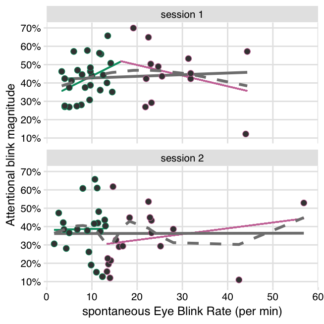
Figure 3.2: No significant relationships between sEBR and AB magnitude in the block before tDCS onset. Grey solid lines show a linear fit over all data points (individual participants), with no clear relationship in both sessions. Grey dashed lines show a cubic spline fit over all data points. Colored lines show two separate linear fits, delimited by the break point in the cubic spline, as estimated with the “two-lines test” (Simonsohn 2018). Both the spline fit and the two linear slopes suggest an Inverted-U shaped relationship in session 1, but neither slope is significant, and this pattern is not present in session 2.
3.3 Relation between sEBR and the effect of tDCS on AB magnitude
r_ABmag_sEBR <- df_sEBR %>%
  left_join(df_ABmag, by = c("subject", "session", "polarity")) %>%
  nest(-polarity,-block) %>% # for each session
  mutate(stats = map(data, ~cor.test(.$sEBR, .$AB_magnitude,
                                     alternative = "two.sided",
                                     method = "pearson"))) %>% # correlate sEBR to AB magnitude
  unnest(map(stats,tidy), .drop = TRUE)
sd_ABmag <- df_ABmag %>%
group_by(polarity,block) %>%
summarise(SD = sd(AB_magnitude))r_ABmag <- df_ABmag %>%
spread(block, AB_magnitude) %>% # separate column of scores for each block
rename(baseline_AB_magnitude = pre) %>% # so we can keep "pre" as separate column
gather(block, AB_magnitude, tDCS, post) %>% # collapse tdcs and post columns
nest(-block,-polarity) %>% # for each tdcs/post block and anodal/cathodal
mutate(stats = map(data, ~cor.test(.$baseline_AB_magnitude, .$AB_magnitude,
alternative = "two.sided",
method = "pearson"))) %>% # correlate blocks
unnest(map(stats,tidy), .drop = TRUE)df_ABmag_change <- df_ABmag %>%
group_by(subject,session,polarity) %>%
summarise(`tDCS - baseline` = AB_magnitude[block == "tDCS"] - AB_magnitude[block == "pre"],
`post - baseline` = AB_magnitude[block == "post"] - AB_magnitude[block == "pre"]) %>%
gather(change, AB_magnitude, `tDCS - baseline`, `post - baseline`) %>%
mutate(change = fct_relevel(change, "tDCS - baseline")) # reorder so this comes firstlCorr_tDCS <- df_sEBR %>%
left_join(df_ABmag_change) %>%
nest(-polarity,-change) %>% # for anodal/cathodal & during/after
mutate(stats = map(data, ~cor.test(.$sEBR, .$AB_magnitude,
alternative = "two.sided",
method = "pearson"))) %>% # correlate sEBR to AB magnitude
unnest(map(stats,tidy), .drop = TRUE) # make output into data frame, drop restlCorr_tDCS_BF <- df_sEBR %>%
left_join(df_ABmag_change) %>%
nest(-polarity,-change) %>% # for anodal/cathodal & during/after
mutate(BF_null = 1 / map_dbl(data, ~extractBF(correlationBF(.$sEBR, .$AB_magnitude),
onlybf = TRUE))) %>% # correlate sEBR to AB magnitude
select(-data)corr_co <- r_ABmag_sEBR %>% # reshape data frame for joining later
select(polarity, block, estimate, parameter) %>% # only keep correlations, and key columns
spread(block, estimate) %>%
gather(block, estimate, tDCS, post) %>% # separate column for subsequent blocks
left_join(r_ABmag, by = c("polarity", "block")) %>% # join with reliability df
rename(r_reliability = estimate.y, r_subsequent = estimate.x, r_baseline = pre) %>%
nest(-polarity, -block) %>% # for each polarity and block
mutate(stats = map(data, ~cocor.dep.groups.overlap(.$r_baseline, .$r_subsequent, .$r_reliability,
n = n_total, return.htest = TRUE))) %>% # compare correlations
# This yields a nested list of 10 different statistical test, for each 4 comparsions
unnest(stats, .drop = TRUE) %>% # peel off first layer
mutate(method = as.character(map(stats, "method"))) %>% # add column identifying lists with this method
filter(method == "Pearson and Filon's z (1898)") %>% # keep only them
select(-method) %>%
unnest(map(stats,tidy), .drop = TRUE) # unnest lists into table# plot_tDCS_corr_labels <- lCorr_tDCS %>%
# left_join(lCorr_tDCS_BF) %>%
# mutate(label = paste0("r(", parameter ,")", " = ", printnum(estimate,gt1=F),
# ", p = ", printp(p.value),
# ", BF = ", round(BF_null,1)))
# separate df so arrows only show on one facet
AB_arrows_y <- tibble(x = c(-16, -16),
xend = c(-16, -16),
y = c(-.05, .05),
yend = c(-.32, .32),
change = factor("tDCS - baseline", levels = levels(df_ABmag_change$change)))
AB_labs_y <- tibble(x = c(-20, -20),
y = c(-.32, .32),
label = c("Smaller AB","Larger AB"),
hjust = c("left","right"),
change = factor("tDCS - baseline", levels = levels(df_ABmag_change$change)))
df_sEBR %>%
left_join(df_ABmag_change) %>%
ggplot(aes(sEBR, AB_magnitude)) +
facet_grid(polarity~change) +
geom_hline(yintercept = 0, linetype = "dashed", color = "gray") +
geom_smooth(aes(color = polarity, linetype = change), method = "lm", show.legend = FALSE) +
geom_point(shape = 21, fill = "gray25", size = 2, color = "white", stroke = .3) +
# geom_label(data = plot_tDCS_corr_labels, aes(label = label), x = 62, y = .3,
# size = geom_text_size, label.size = 0, hjust = "right", vjust = "top") +
scale_color_manual(values = c("#EF7881", "#ABCCE7")) +
scale_x_continuous("spontaneous Eye Blink Rate (per min)", breaks = seq(0,60,10)) +
scale_y_continuous("Change in AB magnitude", breaks = seq(-.3,.3,.1),
labels = scales::percent_format(accuracy = 1)) +
coord_cartesian(xlim = c(0, 60), ylim = c(-.3, .3), clip = "off") +
geom_segment(data = AB_arrows_y, # y-axis arrows
aes(x = x, xend = xend, y = y, yend = yend),
arrow = arrow(angle = 20, length = unit(4,"mm"))) +
geom_text(data = AB_labs_y, # y-axis arrow text
aes(x = x, y = y, label = label, hjust = hjust), size = geom_text_size, angle = 90) +
theme_minimal_grid(font_size = base_font_size, font_family = base_font_family) +
theme(strip.background = element_rect(fill = "grey90"),
panel.spacing = unit(1,"lines"), # add spacing between facets
# move axis labels away from annotatations
axis.title.y = element_text(margin = margin(t = 0, r = 23, b = 0, l = 0))) +
NULL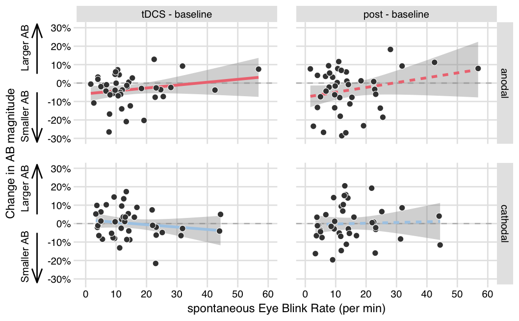
Figure 3.3: No significant relationships between sEBR and AB magnitude change scores. Each plot shows spontaneous eye blink rates on the x-axis, and the change in AB magnitude on the y-axis (difference scores of the tDCS block - the baseline block, or the post block - baseline) in the anodal and cathodal stimulation conditions.
Although there was no relationship between sEBR and AB magnitude itself, sEBR could potentially still be associated with tDCS-induced changes in AB magnitude. We therefore computed AB magnitude change scores (tDCS - baseline, post - baseline) in each stimulation condition (anodal, cathodal), and correlated these to sEBR. However, this analysis did not uncover any significant relationships (Figure 3.3 and columns 2–4 in Table 3.2). We also separately computed the correlations between sEBR and AB magnitude in the baseline block and in the subsequent blocks (Table 3.1). A Pearson-Filon test revealed that these correlations did not differ signifcantly from each other (columns 5–6 in Table 3.1), again suggesting there was no relationship between sEBR and AB magnitude change scores.
ABmag_tbl <- r_ABmag_sEBR %>%
  left_join(sd_ABmag) %>%
  select(polarity,block,estimate,SD) %>%
  mutate(block = factor(block, levels = c("pre","tDCS","post")),
         block = fct_recode(block, baseline = "pre")) %>% # reorder so this comes first)
  arrange(polarity,block) %>%
  select(block,estimate,SD)

ABmag_tbl %>%
  kable(col.names = c("Block",
                      paste0("$r$ sEBR", footnote_marker_alphabet(1)),
                      paste0("SD", footnote_marker_alphabet(2))),
        caption = "Variability of attentional blink magnitude scores and correlation with sEBR, per stimulation condition and block.",
        booktabs = TRUE,
        digits = 3,
        escape = FALSE) %>%
  kable_styling() %>%
  pack_rows(index = c("anodal session" = 3, "cathodal session" = 3)) %>%
  column_spec(1, width = "10em") %>%
  footnote(escape = FALSE, threeparttable = TRUE, alphabet = c(
    "Pearson's correlation between AB magnitude and spontaneous eye blink rate",
"Standard deviation of AB magnitude"))| Block | \(r\) sEBRa | SDb |
|---|---|---|
| anodal session | ||
| baseline | 0.037 | 0.140 |
| tDCS | 0.151 | 0.148 |
| post | 0.249 | 0.137 |
| cathodal session | ||
| baseline | 0.046 | 0.136 |
| tDCS | -0.053 | 0.128 |
| post | 0.086 | 0.120 |
| a Pearson’s correlation between AB magnitude and spontaneous eye blink rate | ||
| b Standard deviation of AB magnitude | ||
corr_co_tbl <- corr_co %>%
  select(polarity, change = "block", Z = "statistic", p = "p.value", r_reliability = "estimate3") %>%
  mutate(change = factor(change), # make equal to other data frame
         change = fct_recode(change,  `tDCS - baseline` = "tDCS", `post - baseline` = "post"),
         change = fct_relevel(change, "tDCS - baseline")) %>%
  left_join(lCorr_tDCS, by = c("polarity", "change")) %>% # Pearson correlations difference scores
  left_join(lCorr_tDCS_BF, by = c("polarity", "change")) %>% # Bayesian correlations difference scores
  arrange(polarity) %>% # order rows
  select(change, estimate, p.value, BF_null, Z, p, r_reliability) # order columns

corr_co_tbl %>%
  kable(col.names = c("contrast","$r$","$p$","$BF_{01}$","$Z$","$p$","$r$"),
        digits = 3,
        caption = "Attentional blink magnitude and spontaneous eye blink rate correlations.",
        booktabs = TRUE,
        escape = FALSE) %>%
  kable_styling() %>%
  pack_rows(index = c("anodal session" = 2, "cathodal session" = 2)) %>%
  add_header_above(setNames(c(1,3,2,1), c(" ",
              paste0("Correlation", footnote_marker_alphabet(1, double_escape = TRUE)),
              paste0("Pearson-Filon test", footnote_marker_alphabet(2, double_escape = TRUE)),
              paste0("Reliability", footnote_marker_alphabet(3, double_escape = TRUE)))),
                   escape = FALSE) %>%
  footnote(escape = FALSE, threeparttable = TRUE, alphabet = c(
    "Linear correlation (Pearson and Bayesian) between sEBR and AB magnitude change scores",
    "Test for significant differences between the sEBR vs. AB magnitude correlations (reported in Table \\3.1) in the baseline vs. tDCS or post blocks",
"Pearson correlation between AB magnitude scores in the baseline vs. tDCS or post blocks"))| contrast | \(r\) | \(p\) | \(BF_{01}\) | \(Z\) | \(p\) | \(r\) |
|---|---|---|---|---|---|---|
| anodal session | ||||||
| tDCS - baseline | 0.208 | 0.199 | 1.371 | -1.269 | 0.204 | 0.836 |
| post - baseline | 0.241 | 0.133 | 1.053 | -1.592 | 0.111 | 0.629 |
| cathodal session | ||||||
| tDCS - baseline | -0.164 | 0.313 | 1.812 | 1.046 | 0.296 | 0.818 |
| post - baseline | 0.040 | 0.808 | 2.766 | -0.326 | 0.745 | 0.706 |
| a Linear correlation (Pearson and Bayesian) between sEBR and AB magnitude change scores | ||||||
| b Test for significant differences between the sEBR vs. AB magnitude correlations (reported in Table 3.1) in the baseline vs. tDCS or post blocks | ||||||
| c Pearson correlation between AB magnitude scores in the baseline vs. tDCS or post blocks | ||||||
4 Discussion
Dopamine levels play a central role in regulating cognitive functions. tDCS may be used to enhance cognitive functions, but its precise effects appear to be dependent on dopamine as well. Here we attempted to use sEBR—a proxy for dopaminergic activity—to study how dopamine may determine the size of the AB and its modulation by tDCS. As a prerequisite, we assessed the test-retest reliabilities of sEBR and AB magnitude, which proved to be good to moderate, respectively, in line with previous reports (Kruis et al. 2016; Dang et al. 2017; Dale, Dux, and Arnell 2013). We then attempted to replicate a result from Colzato et al. (2008), who reported that individuals with high sEBR tend to exhibit a smaller AB. However, we found no significant linear or Inverted-U-shaped relationship between sEBR and AB magnitude, with more evidence for the null hypothesis of no association. Finally, we also did not find any evidence that sEBR is associated with the effects of tDCS on AB magnitude.
4.1 sEBR and AB magnitude have good to moderate test-retest reliability
The test-retest reliability of sEBR across two testing sessions (separated by about one week) was “good”, bordering on “excellent” (Koo and Li 2016). Only two other studies examined the reliability of sEBR to date. Dang et al. (2017) (n = 18) found a Pearson correlation of .86 between sEBR under administration of bromocriptine (a dopamine agonist) or placebo (separated by 4 hours). Here, Pearson’s correlation was comparable (.84). In Kruis et al. (2016), Cronbach’s alpha for sEBR ranged from .85 (three measurements of 27 long-term meditators) to .79 (2–3 measurements of 114 meditation-naive participants). In our data, Cronbach’s alpha was even slightly higher (.91). Together, all three studies suggest that sEBR scores are trait-like and stable over time, even for short measurements of only several minutes (6 minutes here and in Kruis et al. (2016); 5 minutes in Dang et al. (2017)). Although the reliability estimates are comparable, we measured sEBR twice under baseline conditions, whereas Dang et al. (2017) administered a dopamine agonist in one measurement (vs. placebo), and Kruis et al. (2016) measured sEBR following meditation practice (vs. a regular day). We did find that participants with prior EEG experience exhibited a two- to threefold lower sEBR. Future studies that measure sEBR with EEG electrodes might want to take this into account. However, this observation was based on only 6 participants, and sEBR did not significantly differ between sessions, despite the fact that all participants had EEG experience after the first session.
In contrast to sEBR, AB magnitude was significantly smaller in the second session. Previous studies have reported that performance on an AB task can improve across sessions (Dale, Dux, and Arnell 2013; Slagter et al. 2007), but for targets at all lags, whereas here we observed a specific increase in lag 3 T2|T1 performance (inside the attentional blink window). Test-retest reliability of AB magnitude was lower than sEBR: the point-estimate indicated only “moderate” reliability, though the 95% confidence interval was also consistent with “poor” to “good” reliability. However, this is comparable to previous reports (see Table 4.1). The Pearson correlation in the present study (r = .68) is even on the higher end of the range reported in previous studies (though note that regular correlations can overestimate “true” test-retest reliability (Bland and Altman 1986)).
The moderate reliability for AB magnitude limits the correlation that can be obtained between AB magnitude and sEBR. The AB phenomenon might suffer from the “individual differences paradox” (Hedge, Powell, and Sumner 2018): precisely because it is robust at the group level (almost everyone has an AB), it might not exhibit sufficient between-subject variability to be reliable. On the other hand, the AB seems to have a larger range of individual differences than other tasks (Willems and Martens 2016), and even a moderate reliability should provide “enough room” to detect correlations between sEBR and AB magnitude in a plausible range.
| Study | n | Correlation | Notes |
|---|---|---|---|
| Kelly and Dux (2011) | 37 | .33, .34, .48, .52, | test and retest on same day; different values correspond to different tasks |
| Dale and Arnell (2013) | 46 | .62, .39 | test and retest one week apart; 1st value is a task with a set-switch, 2nd is without |
| Dale, Dux, and Arnell (2013) | 118 | .41, .41, .45, .48, .49 | test and retest one week apart; different values correspond to different tasks |
| London and Slagter (2015) | 34 | .58 | test and retest one week apart; almost same task as present study |
4.2 No significant relationships between sEBR and baseline AB magnitude
ABmag_mean <- mean(df_ABmag$AB_magnitude[df_ABmag$block == "pre"])
ABmag_best <- min(df_ABmag$AB_magnitude[df_ABmag$block == "pre"])
Colzato et al. (2008) (n = 20) found a negative correlation between sEBR and AB magnitude. Here, this correlation was not significant in either session, with an effect size around 0 (session 2) or even slightly positive (session 1). The main difference between both studies seems to be the distribution of AB magnitude scores. The AB was shallow in Colzato et al. (2008), as average AB magnitude was less than 10%, with 5 out of 20 participants showing either a “negative” AB (higher T2|T1 accuracy at the shortest lag) or an AB magnitude around 0. Here, the blink was much more pronounced (40% on average)—even the best performing participant had an AB magnitude (11%) that exceeded the average in Colzato et al. (2008).
Our AB task also involves an attentional set switch, while the task used by Colzato et al. (2008) did not. In our task, T1 and T2 had different features (T1 was red; T2 was green), so participants had to update their attentional template and detect the second target on the basis of a different feature (color) than T1. In Colzato et al. (2008), T1 and T2 were both digits, and thus belonged to the same set. Kelly and Dux (2011) suggest that such a set switch introduces an additional bottle neck that is dissociable from the AB (Potter et al. 1998). However, follow-up studies have shown that there is still a sizable correlation between non-switch and switch-versions of AB tasks (Dale, Dux, and Arnell 2013; Dale and Arnell 2013). Although a set switch may introduce additional variance, it seems unlikely this would be sufficient to completely abolish a correlation between sEBR and AB magnitude. However, it could have reduced the size of the effect to a degree where it could no longer be reliably detected. The correlation between sEBR and AB magnitude in Colzato et al. (2008) (r = -.53) appears to exceed the average reliability of AB magnitude itself (Table 4.1), suggesting it might be an overestimate of the true correlation. Further evidence that the effect might be small comes from Unsworth, Robison, and Miller (2019), who conducted a large-scale study (n = 204) and only found a correlation of .17 between sEBR and attentional control (psychomotor vigilance task, antisaccade task), and no correlation with working memory (operation, symmetry, and reading span)—a core component in the AB (Dux and Marois 2009; Martens and Wyble 2010). Although our sample size is twice that of Colzato et al. (2008), an effect of this magnitude would not have been detectable. It should also be noted that we used almost the same task as Slagter and Georgopoulou (2013) (n = 39), who also did not find a significant correlation between sEBR and AB magnitude. So both our studies do not support a relationship between sEBR and the AB.
No study to date has investigated an Inverted-U-shaped relationship between sEBR and AB magnitude, even though the underlying theory strongly suggests it (Cools and D’Esposito 2011; Slagter et al. 2012). Here the data do conform to a weak Inverted-U-shaped relationship, but only in session 1, and neither the upward nor the downward slope were significantly different from 0. Because both would have to be significant (Simonsohn 2018), and each slope is estimated on a different subset of the sample, we likely did not have sufficient power to detect an Inverted-U-shaped relationship. To be able to detect an Inverted-U-shaped relationship, the participants in our sample should also cover the whole range of AB task performance and dopamine levels. If this assumption is not met, then a true Inverted-U-shaped relationship could also masquerade as a linear effect (if all participants are sub-optimal), or no effect (if all participants are in the optimal range).
Two recent studies have cast doubt on the validity of sEBR as proxy for striatal dopamine. Both used PET to measure dopamine non-invasively in humans, but found no relation between sEBR and striatal dopamine receptor availability (Dang et al. 2017) or dopamine synthesis capacity (Sescousse et al. 2018). So, even though we find no relation between sEBR and the AB, there could still be a true relationship between dopamine and the AB—sEBR might simply not have high validity to measure it accurately.
4.3 No significant relationship between sEBR and the effect of tDCS on AB magnitude
We suggested two factors that might underlie individual differences in the effects of tDCS on the AB (See Figure 1.1). First, baseline cortical excitability might partially determine whether tDCS leads to behavioral improvements or impairments (Krause, Márquez-Ruiz, and Cohen Kadosh 2013) (Figure 1.1, left panel). This seems to fit the results of London and Slagter (2015), who found that individuals that benefitted from anodal tDCS tended to worsen with cathodal tDCS (and vice versa). However, we did not replicate this negative correlation between the effects of anodal and cathodal tDCS (see Reteig et al. 2019b), so this finding may not be robust.
Second, baseline dopamine levels may also partially determine the behavioral effects of tDCS (Wiegand, Nieratschker, and Plewnia 2016) (Figure 1.1, right panel). Assuming that sEBR is a valid index of dopamine levels, we found no evidence for this result, though our Bayes Factor analyses also did not indicate strong evidence of absence. The model proposed by Wiegand, Nieratschker, and Plewnia (2016) is based on just two studies (Plewnia et al. 2013; Nieratschker et al. 2015) that show different effects of tDCS in different COMT-subtypes, who should vary in baseline dopamine levels. However, a more recent study found that offline effects of prefrontal tDCS on working memory did not interact with COMT genotype (Jongkees et al. 2018). Because tDCS may itself also boost dopamine release in the striatum (Tanaka et al. 2013; Fonteneau et al. 2018), the model is complicated even further. On a more basic level, it is also still disputed whether the COMT polymorphism can affect cognitive functioning (Barnett, Scoriels, and Munafò 2008), as most studies are likely severely underpowered (Border et al. 2019). The only study that looked at the relation between COMT and the AB also found no association (Colzato et al. 2011), although this was a very small study for genotyping standards. Thus, the overall evidence that the effect of tDCS on the AB depends on baseline dopamine levels is preliminary.
Finally, it is unclear how both axes of the model (Figure 1.1) relate to each other. Pairing tDCS with dopaminergic drugs produces complex and non-linear effects on cortical excitability (Monte-Silva et al. 2009; Fresnoza et al. 2014). Two studies that have combined tDCS and administration of tyrosine (a dopamine precursor) in cognitive tasks have indeed led to divergent results. Cathodal tDCS of the lDLPFC appears to counteract the beneficial effects of tyrosine, as their combination had no net behavioral effect (Jongkees et al. 2017; Dennison et al. 2018). In contrast, combining anodal tDCS with tyrosine led to impaired performance on an n-back task, where anodal tDCS alone would be expected to enhance performance (Jongkees et al. 2017). Future studies that manipulate both dopamine levels and cortical excitability are necessary to uncover the physiology that could lead to such interactions.
4.4 Conclusions
We found that spontaneous eye blink rate is a reliable measure, but that it does not relate to the attentional blink, or to changes in attentional blink size following tDCS. Because dopamine is central to healthy cognitive and brain function, it remains plausible that dopamine interacts with manipulations of brain function, such as tDCS, as well as cognitive tasks such as the AB. But there is no good prior for how large the influence of dopamine is. Considering the large individual variability in AB size (Willems and Martens 2016), and the many factors that play a role in tDCS outcome (Li, Uehara, and Hanakawa 2015; Krause and Cohen Kadosh 2014), dopamine might account for only a small portion of the total variability. In addition, sEBR only provides an indirect measure of dopamine function, and this has recently also been questioned (Dang et al. 2017; Sescousse et al. 2018). More large-scale studies that include more direct measurement (e.g., using ligand-PET) or manipulation (e.g., using pharmacology) of dopamine function will be needed to pinpoint the unique contribution of dopamine.
Acknowledgements
This work was supported by a Research Talent Grant from the Netherlands Organization for Scientific Research (NWO) (452-10-018, to HAS and KRR). We thank Raquel London for sharing all her experience and materials, as well as Daphne Box and Esther van der Giessen for their assistance in data collection.
References
r_refs(file = "r-references.bib")Aust, Frederik, and Marius Barth. 2018. papaja: Create APA Manuscripts with R Markdown. https://github.com/crsh/papaja.
Barbato, Giuseppe, Gianluca Ficca, Giovanni Muscettola, Mariateresa Fichele, Michele Beatrice, and Franco Rinaldi. 2000. “Diurnal variation in spontaneous eye-blink rate.” Psychiatry Research 93 (2): 145–51. https://doi.org/10.1016/S0165-1781(00)00108-6.
Barnett, Jennifer H., Linda Scoriels, and Marcus R. Munafò. 2008. “Meta-Analysis of the Cognitive Effects of the Catechol-O-Methyltransferase Gene Val158/108Met Polymorphism.” Biological Psychiatry 64 (2): 137–44. https://doi.org/10.1016/j.biopsych.2008.01.005.
Bestmann, Sven, Archy O. De Berker, and James Bonaiuto. 2015. “Understanding the behavioural consequences of noninvasive brain stimulation.” Trends in Cognitive Sciences 19 (1). Elsevier Ltd: 13–20. https://doi.org/10.1016/j.tics.2014.10.003.
Bindman, Lynn J, O C J Lippold, and J W T Redfearn. 1964. “The action of brief polarizing currents on the cerebral cortex of the rat (1) during current flow and (2) in the production of long-lasting after effects.” Journal of Physiology 172: 369–82. https://doi.org/10.1113/jphysiol.1964.sp007425.
Björklund, Anders, and Stephen B Dunnett. 2007. “Dopamine neuron systems in the brain: an update.” Trends in Neurosciences 30 (5): 194–202. https://doi.org/10.1016/j.tins.2007.03.006.
Bland, J Martin, and Douglas G Altman. 1986. “Statistical methods for assessing agreement between two methods of clinical measurement.” The Lancet 327: 307–10. https://doi.org/10.1016/S0140-6736(86)90837-8.
Border, Richard, Emma C. Johnson, Luke M. Evans, Andrew Smolen, Noah Berley, Patrick F. Sullivan, and Matthew C. Keller. 2019. “No Support for Historical Candidate Gene or Candidate Gene-by-Interaction Hypotheses for Major Depression Across Multiple Large Samples.” American Journal of Psychiatry. https://doi.org/10.1176/appi.ajp.2018.18070881.
Caffier, Philipp P., Udo Erdmann, and Peter Ullsperger. 2003. “Experimental evaluation of eye-blink parameters as a drowsiness measure.” European Journal of Applied Physiology 89 (3-4): 319–25. https://doi.org/10.1007/s00421-003-0807-5.
Cohen, J. D., G. Aston-Jones, and M. S. Gilzenrat. 2004. “A Systems-Level Perspective on Attention and Cognitive Control: Guided Activation, Adaptive Gating, Conflict Monitoring, and Exploitation versus Exploration.” In Cognitive Neuroscience of Attention, edited by Michael I Posner, 71–90. New York, NY, US: The Guilford Press.
Colzato, Lorenza S, Heleen A Slagter, Michiel M A Spapé, and Bernhard Hommel. 2008. “Blinks of the eye predict blinks of the mind.” Neuropsychologia 46 (13): 3179–83. https://doi.org/10.1016/j.neuropsychologia.2008.07.006.
Colzato, LS, HA Slagter, Mischa De Rover, and Bernhard Hommel. 2011. “Dopamine and the Management of Attentional Resources: Genetic Markers of Striatal D2 Dopamine Predict Individual Differences in the Attentional Blink.” Journal of Cognitive Neuroscience 23 (11): 3576–85. http://bernhard-hommel.eu/Colzato{\_}AB{\_}genetic.pdf.
Cools, Roshan, and Mark D’Esposito. 2011. “Inverted-U–Shaped Dopamine Actions on Human Working Memory and Cognitive Control.” Biological Psychiatry 69 (12): e113–e125. https://doi.org/10.1016/j.biopsych.2011.03.028.
Dale, Gillian, and Karen M. Arnell. 2013. “How reliable is the attentional blink? Examining the relationships within and between attentional blink tasks over time.” Psychological Research 77 (2): 99–105. https://doi.org/10.1007/s00426-011-0403-y.
Dale, Gillian, Paul E Dux, and Karen M Arnell. 2013. “Individual differences within and across attentional blink tasks revisited.” Attention, Perception & Psychophysics 75 (3): 456–67. https://doi.org/10.3758/s13414-012-0415-8.
Dang, Linh C., Gregory R. Samanez-Larkin, Jaime J. Castrellon, Scott F. Perkins, Ronald L. Cowan, Paul A. Newhouse, and David H. Zald. 2017. “Spontaneous Eye Blink Rate (EBR) Is Uncorrelated with Dopamine D2 Receptor Availability and Unmodulated by Dopamine Agonism in Healthy Adults.” eNeuro 4 (5): ENEURO.0211–17.2017. https://doi.org/10.1523/eneuro.0211-17.2017.
Delorme, Arnaud, and Scott Makeig. 2004. “EEGLAB: an open source toolbox for analysis of single-trial EEG dynamics including independent component analysis.” Journal of Neuroscience Methods 134 (1): 9–21. https://doi.org/10.1016/j.jneumeth.2003.10.009.
Dennison, Olivia, Jie Gao, Lee Wei Lim, Charlotte J Stagg, and Luca Aquili. 2018. “Catecholaminergic modulation of indices of cognitive flexibility: A pharmaco-tDCS study.” Brain Stimulation 12 (2). Elsevier Ltd: 290–95. https://doi.org/https://doi.org/10.1016/j.brs.2018.12.001.
Diedenhofen, Birk, and Jochen Musch. 2015. “Cocor: A Comprehensive Solution for the Statistical Comparison of Correlations.” PLoS ONE 10 (4). Public Library of Science: e0121945. https://doi.org/10.1371/journal.pone.0121945.
Doughty, Michael J., and Taher Naase. 2006. “Further analysis of the human spontaneous eye blink rate by a cluster analysis-based approach to categorize individuals with ’normal’ versus ’frequent’ eye blink activity.” Eye and Contact Lens 32 (6): 294–99. https://doi.org/10.1097/01.icl.0000224359.32709.4d.
Dux, Paul E., and René Marois. 2009. “The attentional blink: A review of data and theory.” Attention, Perception, and Psychophysics 71 (8): 1683–1700. https://doi.org/10.3758/APP.71.8.1683.
Dux, Paul E, and René Marois. 2008. “Distractor inhibition predicts individual differences in the attentional blink.” Edited by Alex O. Holcombe. PloS One 3 (10). Public Library of Science: e3330. https://doi.org/10.1371/journal.pone.0003330.
Fonteneau, Clara, Jérome Redoute, Frédéric Haesebaert, Didier Le Bars, Nicolas Costes, Marie-Françoise Suaud-Chagny, and Jérome Brunelin. 2018. “Frontal Transcranial Direct Current Stimulation Induces Dopamine Release in the Ventral Striatum in Human.” Cerebral Cortex 28 (7): 2636–46. https://doi.org/10.1093/cercor/bhy093.
Fresnoza, Shane, Walter Paulus, Michael A Nitsche, and M.-F. Kuo. 2014. “Nonlinear Dose-Dependent Impact of D1 Receptor Activation on Motor Cortex Plasticity in Humans.” Journal of Neuroscience 34 (7): 2744–53. https://doi.org/10.1523/JNEUROSCI.3655-13.2014.
Gardner, RC, and RWJ Neufeld. 1987. “Use of the simple change score in correlational analyses.” Educational and Psychological Measurement, 849–64.
Gebodh, Nigel, Zeinab Esmaeilpour, Marom Bikson, Devin Adair, Felipe Fregni, and Pedro Schestattsky. 2019. “Transcranial direct current stimulation among technologies for low-intensity transcranial electrical stimulation: classification, history, and terminology.” In Practical Guide to Transcranial Direct Current Stimulation, edited by Helena Knotkova, Michael A. Nitsche, Marom Bikson, and Adam J. Woods, 3–43. Cham (Switzerland): Springer. https://doi.org/10.1007/978-3-319-95948-1_1.
Gibbs, Ayana A., Kris H. Naudts, Edgar P. Spencer, and Anthony S. David. 2007. “The role of dopamine in attentional and memory biases for emotional information.” American Journal of Psychiatry 164 (10): 1603–9. https://doi.org/10.1176/appi.ajp.2007.06081241.
Griffin, Dale, Sandra Murray, and Richard Gonzalez. 1999. “Difference score correlations in relationship research: A conceptual primer.” Personal Relationships 6 (4): 505–18. https://doi.org/10.1111/j.1475-6811.1999.tb00206.x.
Grolemund, Garrett, and Hadley Wickham. 2011. “Dates and Times Made Easy with lubridate.” Journal of Statistical Software 40 (3): 1–25. http://www.jstatsoft.org/v40/i03/.
Hedge, Craig, Georgina Powell, and Petroc Sumner. 2018. “The reliability paradox: Why robust cognitive tasks do not produce reliable individual differences.” Behavior Research Methods 50 (3). Behavior Research Methods: 1166–86. https://doi.org/10.3758/s13428-017-0935-1.
Jongkees, Bryant J., and Lorenza S. Colzato. 2016. “Spontaneous eye blink rate as predictor of dopamine-related cognitive function—A review.” Neuroscience and Biobehavioral Reviews 71. Elsevier Ltd: 58–82. https://doi.org/10.1016/j.neubiorev.2016.08.020.
Jongkees, Bryant J., Alexandra A. Loseva, Fatemeh B. Yavari, Michael A. Nitsche, and Lorenza S. Colzato. 2018. “The COMT Val158Met polymorphism does not modulate the after-effect of tDCS on working memory.” European Journal of Neuroscience, no. July 2018: 263–74. https://doi.org/10.1111/ejn.14261.
Jongkees, Bryant J., Roberta Sellaro, Christian Beste, Michael A. Nitsche, Simone Kühn, and Lorenza S. Colzato. 2017. “L-Tyrosine administration modulates the effect of transcranial direct current stimulation on working memory in healthy humans.” Cortex 90: 103–14. https://doi.org/10.1016/j.cortex.2017.02.014.
Käenmäki, Mikko, Anne Tammimäki, Timo Myöhänen, Kaisa Pakarinen, Carolina Amberg, Maria Karayiorgou, Joseph A. Gogos, and Pekka T. Männistö. 2010. “Quantitative role of COMT in dopamine clearance in the prefrontal cortex of freely moving mice.” Journal of Neurochemistry 114 (6): 1745–55. https://doi.org/10.1111/j.1471-4159.2010.06889.x.
Kelly, Ashleigh J., and Paul E. Dux. 2011. “Different Attentional Blink Tasks Reflect Distinct Information Processing Limitations: An Individual Differences Approach.” Journal of Experimental Psychology: Human Perception and Performance 37 (6): 1867–73. https://doi.org/10.1037/a0025975.
Klein, C., B. Andresen, and E. Thom. 1993. “Blinking, alpha brain waves and smoking in schizophrenia.” Acta Psychiatrica Scandinavica 87 (3): 172–78. https://doi.org/10.1111/j.1600-0447.1993.tb03351.x.
Koo, Terry K., and Mae Y. Li. 2016. “A Guideline of Selecting and Reporting Intraclass Correlation Coefficients for Reliability Research.” Journal of Chiropractic Medicine 15 (2). Elsevier B.V.: 155–63. https://doi.org/10.1016/j.jcm.2016.02.012.
Krause, Beatrix, and Roi Cohen Kadosh. 2014. “Not all brains are created equal: the relevance of individual differences in responsiveness to transcranial electrical stimulation.” Frontiers in Systems Neuroscience 8 (February): 25. https://doi.org/10.3389/fnsys.2014.00025.
Krause, Beatrix, Javier Márquez-Ruiz, and Roi Cohen Kadosh. 2013. “The effect of transcranial direct current stimulation: a role for cortical excitation/inhibition balance?” Frontiers in Human Neuroscience 7 (September): 602. https://doi.org/10.3389/fnhum.2013.00602.
Kruis, Ayla, Heleen A. Slagter, David R.W. Bachhuber, Richard J. Davidson, and Antoine Lutz. 2016. “Effects of meditation practice on spontaneous eyeblink rate.” Psychophysiology 53 (5): 749–58. https://doi.org/10.1111/psyp.12619.
Kuo, Min Fang, Walter Paulus, and Michael A. Nitsche. 2008. “Boosting focally-induced brain plasticity by dopamine.” Cerebral Cortex 18 (3): 648–51. https://doi.org/10.1093/cercor/bhm098.
Li, Lucia M., Kazumasa Uehara, and Takashi Hanakawa. 2015. “The contribution of interindividual factors to variability of response in transcranial direct current stimulation studies.” Frontiers in Cellular Neuroscience 9 (May): 181. https://doi.org/10.3389/fncel.2015.00181.
Liu, Anli, Mihály Vöröslakos, Greg Kronberg, Simon Henin, Matthew R. Krause, Yu Huang, Alexander Opitz, et al. 2018. “Immediate neurophysiological effects of transcranial electrical stimulation.” Nature Communications 9 (1). Springer US: 5092. https://doi.org/10.1038/s41467-018-07233-7.
London, Raquel E., and Heleen A Slagter. 2015. “Effects of transcranial direct current stimulation over left dorsolateral PFC on the attentional blink depend on individual baseline performance.” Journal of Cognitive Neuroscience 27 (12): 2382–93. https://doi.org/10.1162/jocn_a_00867.
Luck, Steven J. 2005. An Introduction to the Event-Related Potential Technique. Vol. 36. 6. Cambridge, MA: MIT Press.
Ly, Alexander, Josine Verhagen, and Eric Jan Wagenmakers. 2016. “Harold Jeffreys’s default Bayes factor hypothesis tests: Explanation, extension, and application in psychology.” Journal of Mathematical Psychology 72. Elsevier Inc.: 19–32. https://doi.org/10.1016/j.jmp.2015.06.004.
Martens, Sander, Jaap Munneke, Hendrikus Smid, and Addie Johnson. 2006. “Quick Minds Don’t Blink: Electrophysiological Correlates of Individual Differences in Attentional Selection.” Journal of Cognitive Neuroscience 18 (9): 1423–38. https://doi.org/10.1162/jocn.2006.18.9.1423.
Martens, Sander, and Brad Wyble. 2010. “The attentional blink: Past, present, and future of a blind spot in perceptual awareness.” Neuroscience and Biobehavioral Reviews 34 (6). Elsevier Ltd: 947–57. https://doi.org/10.1016/j.neubiorev.2009.12.005.
Matsuo, Fumisuke, Jon F. Peters, and Edward L. Reilly. 1975. “Electrical phenomena associated with movements of the eyelid.” Electroencephalography and Clinical Neurophysiology 38 (5): 507–11. https://doi.org/10.1016/0013-4694(75)90191-1.
McGraw, Kenneth O., and S. P. Wong. 1996. “Forming inferences about some intraclass correlations coefficients.” Psychological Methods 1 (1): 30–46. https://doi.org/10.1037/1082-989X.1.4.390.
Monte-Silva, K., M.-F. Kuo, N. Thirugnanasambandam, D. Liebetanz, W. Paulus, and M. A. Nitsche. 2009. “Dose-Dependent Inverted U-Shaped Effect of Dopamine (D2-Like) Receptor Activation on Focal and Nonfocal Plasticity in Humans.” Journal of Neuroscience 29 (19): 6124–31. https://doi.org/10.1523/JNEUROSCI.0728-09.2009.
Morey, Richard D., and Jeffrey N. Rouder. 2018. BayesFactor: Computation of Bayes Factors for Common Designs. https://CRAN.R-project.org/package=BayesFactor.
Müller, Kirill. 2017. Here: A Simpler Way to Find Your Files. https://CRAN.R-project.org/package=here.
Nieoullon, A. 2002. “Dopamine and the regulation of cognition and attention.” Progress in Neurobiology 67: 53–83.
Nieratschker, Vanessa, Christoph Kiefer, Katrin Giel, Rejko Kruger, and Christian Plewnia. 2015. “The COMT Val/Met polymorphism modulates effects of tDCS on response inhibition.” Brain Stimulation 8 (2): 283–88. https://doi.org/10.1016/j.brs.2014.11.009.
Nitsche, Michael A., Christian Lampe, Andrea Antal, David Liebetanz, Nicolas Lang, Frithjof Tergau, and Walter Paulus. 2006. “Dopaminergic modulation of long-lasting direct current-induced cortical excitability changes in the human motor cortex.” European Journal of Neuroscience 23 (6): 1651–7. https://doi.org/10.1111/j.1460-9568.2006.04676.x.
Nitsche, Michael A., and W Paulus. 2000. “Excitability changes induced in the human motor cortex by weak transcranial direct current stimulation.” The Journal of Physiology 527 Pt 3 (2000): 633–9. https://doi.org/10.1111/j.1469-7793.2000.t01-1-00633.x.
Nitsche, Michael A., and W. Paulus. 2001. “Sustained excitability elevations induced by transcranial DC motor cortex stimulation in humans.” Neurology 57 (10): 1899–1901. https://doi.org/10.1212/WNL.57.10.1899.
Parkin, Beth L., Hamed Ekhtiari, and Vincent F. Walsh. 2015. “Non-invasive human brain stimulation in cognitive neuroscience: a primer.” Neuron 87 (5). Elsevier Inc.: 932–45. https://doi.org/10.1016/j.neuron.2015.07.032.
Pearson, K., and L. N. G. Filon. 1898. “Mathematical Contributions to the Theory of Evolution. IV. On the Probable Errors of Frequency Constants and on the Influence of Random Selection on Variation and Correlation.” Philosophical Transactions of the Royal Society A: Mathematical, Physical and Engineering Sciences 191 (0): 229–311. https://doi.org/10.1098/rsta.1898.0007.
Plewnia, Christian, Bastian Zwissler, Isabella Längst, Brigitte Maurer, Katrin Giel, and Rejko Krüger. 2013. “Effects of transcranial direct current stimulation (tDCS) on executive functions: Influence of COMT Val/Met polymorphism.” Cortex 49 (7): 1801–7. https://doi.org/10.1016/j.cortex.2012.11.002.
Potter, Mary C, Marvin M Chun, Bradley S Banks, and Margaret Muckenhoupt. 1998. “Two attentional deficits in serial target search: The visual attentional blink and an amodal task-switch deficit.” Journal of Experimental Psychology: Learning, Memory, and Cognition 24 (4): 979–92.
Purpura, DP, and JG McMurtry. 1965. “Intracellular activities and evoked potential changes during polarization of motor cortex.” Journal of Neurophysiology 28: 166–85.
Raymond, Jane E., Kimron L. Shapiro, and Karen M. Arnell. 1992. “Temporary suppression of visual processing in an RSVP task: An attentional blink?” Journal of Experimental Psychology: Human Perception and Performance 18 (3): 849–60.
R Core Team. 2018. R: A Language and Environment for Statistical Computing. Vienna, Austria: R Foundation for Statistical Computing. https://www.R-project.org/.
Reteig, Leon C., Lionel A. Newman, K. Richard Ridderinkhof, and Heleen A. Slagter. 2019a. “EEG study of the attentional blink; before, during, and after transcranial Direct Current Stimulation (tDCS).”
———. 2019b. “Effects of tDCS on the attentional blink revisited: A statistical evaluation of a replication attempt.”
Revelle, William. 2018. Psych: Procedures for Psychological, Psychometric, and Personality Research. Evanston, Illinois: Northwestern University. https://CRAN.R-project.org/package=psych.
Robbins, T.W., and A.F.T. Arnsten. 2009. “The Neuropsychopharmacology of Fronto-Executive Function: Monoaminergic Modulation.” Annual Review of Neuroscience 32 (1): 267–87. https://doi.org/10.1146/annurev.neuro.051508.135535.
Robinson, David, and Alex Hayes. 2018. Broom: Convert Statistical Analysis Objects into Tidy Tibbles. https://CRAN.R-project.org/package=broom.
RStudio Team. 2016. “RStudio: Integrated Development Environment for R.” Boston, MA: RStudio, Inc. http://www.rstudio.com/.
Schacht, Joseph P. 2016. “COMT val158met moderation of dopaminergic drug effects on cognitive function: a critical review.” The Pharmacogenomics Journal 16 (5): 430–38. https://doi.org/10.1038/tpj.2016.43.
Schultz, Wolfram. 2007. “Multiple Dopamine Functions at Different Time Courses.” Annual Review of Neuroscience 30 (1): 259–88. https://doi.org/10.1146/annurev.neuro.28.061604.135722.
Sescousse, Guillaume, Romain Ligneul, Ruth J. van Holst, Lieneke K. Janssen, Femke de Boer, Marcel Janssen, Anne S. Berry, William J. Jagust, and Roshan Cools. 2018. “Spontaneous eye blink rate and dopamine synthesis capacity: preliminary evidence for an absence of positive correlation.” European Journal of Neuroscience 47 (9): 1081–6. https://doi.org/10.1111/ejn.13895.
Shrout, Patrick E, and Joseph L Fleiss. 1979. “Intraclass correlations: Uses in assessing rater reliability.” Psychological Bulletin 86 (2): 420–28. https://doi.org/10.1037/0033-2909.86.2.420.
Simonsohn, Uri. 2018. “Two Lines: A Valid Alternative to the Invalid Testing of U-Shaped Relationships with Quadratic Regressions.” Advances in Methods and Practices in Psychological Science 1 (4): 538–55. https://doi.org/doi.org/10.1177/251524591880575.
Slagter, H. A., N. C. van Wouwe, K. Kanoff, R. P. P. P. Grasman, D. O. Claassen, W. P. M. van den Wildenberg, and S. A. Wylie. 2016. “Dopamine and temporal attention: An attentional blink study in Parkinson’s disease patients on and off medication.” Neuropsychologia 91. Elsevier: 407–14. https://doi.org/10.1016/j.neuropsychologia.2016.09.006.
Slagter, Heleen A, and Katerina Georgopoulou. 2013. “Distractor inhibition predicts individual differences in recovery from the attentional blink.” PloS One 8 (5): e64681. https://doi.org/10.1371/journal.pone.0064681.
Slagter, Heleen A., Tom Johnstone, Iseult A.M. Beets, and Richard J. Davidson. 2010. “Neural competition for conscious representation across time: An fMRI study.” PLoS ONE 5 (5): e10556. https://doi.org/10.1371/journal.pone.0010556.
Slagter, Heleen A, Antoine Lutz, Lawrence L Greischar, Andrew D Francis, Sander Nieuwenhuis, James M Davis, and Richard J Davidson. 2007. “Mental training affects distribution of limited brain resources.” PLoS Biology 5 (6): e138. https://doi.org/10.1371/journal.pbio.0050138.
Slagter, Heleen A., Ali Mazaheri, Leon C. Reteig, Ruud Smolders, Martijn Figee, Mariska Mantione, P. Richard Schuurman, and Damiaan Denys. 2017. “Contributions of the Ventral Striatum to Conscious Perception: An Intracranial EEG Study of the Attentional Blink.” The Journal of Neuroscience 37 (5): 1081–9. https://doi.org/10.1523/JNEUROSCI.2282-16.2016.
Slagter, Heleen A., Rachel Tomer, Bradley T. Christian, Andrew S. Fox, Lorenza S. Colzato, Carlye R. King, Dhanabalan Murali, and Richard J. Davidson. 2012. “PET evidence for a role for striatal dopamine in the attentional blink: Functional implications.” Journal of Cognitive Neuroscience 24 (9): 1932–40. https://doi.org/10.1162/jocn_a_00255.
Stagg, Charlotte J, and Michael A. Nitsche. 2011. “Physiological basis of transcranial direct current stimulation.” The Neuroscientist 17 (1): 37–53. https://doi.org/10.1177/1073858410386614.
Tanaka, Tomoko, Yuji Takano, Satoshi Tanaka, Naoyuki Hironaka, Kazuto Kobayashi, Takashi Hanakawa, Katsumi Watanabe, and Manabu Honda. 2013. “Transcranial direct-current stimulation increases extracellular dopamine levels in the rat striatum.” Frontiers in Systems Neuroscience 7 (April): 1–8. https://doi.org/10.3389/fnsys.2013.00006.
Unsworth, Nash, Matthew K. Robison, and Ashley L. Miller. 2019. “Individual differences in baseline oculometrics: Examining variation in baseline pupil diameter, spontaneous eye blink rate, and fixation stability.” Cognitive, Affective, & Behavioral Neuroscience, 1–20. https://doi.org/10.3758/s13415-019-00709-z.
Verhagen, Josine, and Eric Jan Wagenmakers. 2014. “Bayesian tests to quantify the result of a replication attempt.” Journal of Experimental Psychology: General 143 (4): 1457–75. https://doi.org/10.1037/a0036731.
Wagenmakers, Eric Jan, Jonathon Love, Maarten Marsman, Tahira Jamil, Alexander Ly, Josine Verhagen, Ravi Selker, et al. 2018. “Bayesian inference for psychology. Part II: Example applications with JASP.” Psychonomic Bulletin and Review 25 (1): 58–76. https://doi.org/10.3758/s13423-017-1323-7.
Wagenmakers, Eric-Jan, Josine Verhagen, and Alexander Ly. 2016. “How to quantify the evidence for the absence of a correlation.” Behavior Research Methods 48. Behavior Research Methods: 413–26. https://doi.org/10.3758/s13428-015-0593-0.
Wickham, Hadley. 2017. Tidyverse: Easily Install and Load the ’Tidyverse’. https://CRAN.R-project.org/package=tidyverse.
Wiegand, Ariane, Vanessa Nieratschker, and Christian Plewnia. 2016. “Genetic Modulation of Transcranial Direct Current Stimulation Effects on Cognition.” Frontiers in Human Neuroscience 10: 651. https://doi.org/10.3389/fnhum.2016.00651.
Wilke, Claus O. 2019. Cowplot: Streamlined Plot Theme and Plot Annotations for ’Ggplot2’. https://github.com/wilkelab/cowplot.
Willems, Charlotte, and Sander Martens. 2016. “Time to see the bigger picture: Individual differences in the attentional blink.” Psychonomic Bulletin and Review 23 (5). Psychonomic Bulletin & Review: 1289–99. https://doi.org/10.3758/s13423-015-0977-2.
Xie, Yihui. 2015. Dynamic Documents with R and Knitr. 2nd ed. Boca Raton, Florida: Chapman; Hall/CRC. https://yihui.name/knitr/.
Xie, Yihui, J. J. Allaire, and Garrett Grolemund. 2018. R Markdown: The Definitive Guide. Boca Raton, FL: CRC Press. https://doi.org/10.1016/B978-0-12-814447-3.00041-0.
Compared to Reteig et al. (2019b), the Participants, Task, and tDCS sections are virtually identical; the Procedure section has been adapted to include the sEBR measurement, the Statistical analysis and sEBR sections are entirely novel.↩
We, furthermore, used the R-packages broom (Version 0.5.1; Robinson and Hayes 2018), cowplot (Version 0.9.99; Wilke 2019), here (Version 0.1; Müller 2017), knitr (Version 1.21; Xie 2015), lubridate (Version 1.7.4; Grolemund and Wickham 2011), papaja (Version 0.1.0.9842; Aust and Barth 2018), and tidyverse (Version 1.2.1; Wickham 2017).↩
FIXME: Insert link↩