library(knitr) # rmarkdown output
library(rmdformats) # r notebook format
library(here) # (relative) file paths
## here() starts at /Volumes/psychology$/Researchers/reteig/AB_tDCS-sEBR## ── Attaching packages ──────────────────────────────────────────────────────────────────────────────────────────────────────────────── tidyverse 1.2.1 ──## ✔ ggplot2 3.1.0 ✔ purrr 0.2.5
## ✔ tibble 2.1.1 ✔ dplyr 0.8.0.1
## ✔ tidyr 0.8.3 ✔ stringr 1.3.1
## ✔ readr 1.1.1 ✔ forcats 0.3.0## Warning: package 'tibble' was built under R version 3.5.2## Warning: package 'tidyr' was built under R version 3.5.2## Warning: package 'dplyr' was built under R version 3.5.2## ── Conflicts ─────────────────────────────────────────────────────────────────────────────────────────────────────────────────── tidyverse_conflicts() ──
## ✖ dplyr::filter() masks stats::filter()
## ✖ dplyr::lag() masks stats::lag()##
## Attaching package: 'psych'## The following objects are masked from 'package:ggplot2':
##
## %+%, alphalibrary(broom) # transform model outputs into data frames
library(BayesFactor) # Bayesian correlations## Loading required package: coda## Loading required package: Matrix##
## Attaching package: 'Matrix'## The following object is masked from 'package:tidyr':
##
## expand## ************
## Welcome to BayesFactor 0.9.12-4.2. If you have questions, please contact Richard Morey (richarddmorey@gmail.com).
##
## Type BFManual() to open the manual.
## ************library(cocor) # significance tests for difference between correlations
source(here("src", "lib", "twolines.R")) # test for U-shaped correlations## Loading required package: nlme##
## Attaching package: 'nlme'## The following object is masked from 'package:dplyr':
##
## collapse## This is mgcv 1.8-24. For overview type 'help("mgcv-package")'.## Loading required package: zoo##
## Attaching package: 'zoo'## The following objects are masked from 'package:base':
##
## as.Date, as.Date.numeric# online: http://webstimate.org/twolines/twolines.R
source(here("src", "lib", "appendixCodeFunctionsJeffreys.R")) # replication Bayes factors## Loading required package: hypergeo## R version 3.5.1 (2018-07-02)
## Platform: x86_64-apple-darwin15.6.0 (64-bit)
## Running under: OS X El Capitan 10.11.6
##
## Matrix products: default
## BLAS: /Library/Frameworks/R.framework/Versions/3.5/Resources/lib/libRblas.0.dylib
## LAPACK: /Library/Frameworks/R.framework/Versions/3.5/Resources/lib/libRlapack.dylib
##
## locale:
## [1] en_US.UTF-8/en_US.UTF-8/en_US.UTF-8/C/en_US.UTF-8/en_US.UTF-8
##
## attached base packages:
## [1] stats graphics grDevices utils datasets methods base
##
## other attached packages:
## [1] hypergeo_1.2-13 lmtest_0.9-36 zoo_1.8-4
## [4] sandwich_2.5-0 mgcv_1.8-24 nlme_3.1-137
## [7] cocor_1.1-3 BayesFactor_0.9.12-4.2 Matrix_1.2-14
## [10] coda_0.19-2 broom_0.5.1 psych_1.8.10
## [13] forcats_0.3.0 stringr_1.3.1 dplyr_0.8.0.1
## [16] purrr_0.2.5 readr_1.1.1 tidyr_0.8.3
## [19] tibble_2.1.1 ggplot2_3.1.0 tidyverse_1.2.1
## [22] here_0.1 rmdformats_0.3.3 knitr_1.21
##
## loaded via a namespace (and not attached):
## [1] httr_1.3.1 jsonlite_1.6 elliptic_1.3-9
## [4] modelr_0.1.2 gtools_3.8.1 shiny_1.2.0
## [7] assertthat_0.2.0 highr_0.7 cellranger_1.1.0
## [10] yaml_2.2.0 pillar_1.3.1 backports_1.1.3
## [13] lattice_0.20-35 glue_1.3.0 digest_0.6.18
## [16] promises_1.0.1 rvest_0.3.2 colorspace_1.3-2
## [19] htmltools_0.3.6 httpuv_1.4.5 plyr_1.8.4
## [22] pkgconfig_2.0.2 haven_1.1.2 questionr_0.6.3
## [25] bookdown_0.9 xtable_1.8-4 mvtnorm_1.0-8
## [28] scales_1.0.0 later_0.7.5 MatrixModels_0.4-1
## [31] generics_0.0.2 withr_2.1.2 pbapply_1.3-4
## [34] lazyeval_0.2.1 cli_1.0.1 mnormt_1.5-5
## [37] magrittr_1.5 crayon_1.3.4 readxl_1.1.0
## [40] mime_0.6 evaluate_0.12 MASS_7.3-50
## [43] xml2_1.2.0 foreign_0.8-70 tools_3.5.1
## [46] hms_0.4.2 munsell_0.5.0 compiler_3.5.1
## [49] contfrac_1.1-12 rlang_0.3.4 grid_3.5.1
## [52] rstudioapi_0.8 miniUI_0.1.1.1 rmarkdown_1.11
## [55] gtable_0.2.0 deSolve_1.21 R6_2.3.0
## [58] lubridate_1.7.4 rprojroot_1.3-2 stringi_1.2.4
## [61] parallel_3.5.1 Rcpp_1.0.0 tidyselect_0.2.5
## [64] xfun_0.4Prepare data
Attentional blink
Read data files
Load the single-trial attentional blink data. First create a list of files:
data_path <- here("data","AB") # top-level folder with task data
# list all the .txt files in folders of individual subjects
files <- dir(data_path, pattern = "*.txt", recursive = TRUE)
head(files,15)
## [1] "S01/AB_S01_1B_post.txt" "S01/AB_S01_1B_pre.txt"
## [3] "S01/AB_S01_1B_tDCS.txt" "S01/AB_S01_2D_post.txt"
## [5] "S01/AB_S01_2D_pre.txt" "S01/AB_S01_2D_tDCS.txt"
## [7] "S02/AB_S02_1D_post.txt" "S02/AB_S02_1D_pre.txt"
## [9] "S02/AB_S02_1D_tDCS.txt" "S02/AB_S02_2B_post.txt"
## [11] "S02/AB_S02_2B_pre.txt" "S02/AB_S02_2B_tDCS.txt"
## [13] "S02/AB_S02_2B_tDCS2.txt" "S03/AB_S03_1D_post.txt"
## [15] "S03/AB_S03_1D_pre.txt"The data for each participant are in a separate folder, containing multiple .txt files, named in the following way: "AB_SUBJECTID_SESSION POLARITY_BLOCK.txt", where:
SUBJECTIDis the same as the folder name (e.g. “S01”, “S47”)SESSIONis either 1 (first session) or 2 (second session)POLARITYis the code for which tDCS polarity was received during this session (anodal or cathodal).- anodal is coded as ‘B’ from S01–S21 and ‘D’ from S22 onwards.
- cathodal is coded as ‘D’ from S01–S21 and ‘I’ from S22 onwards.
BLOCKis whether the data is from the block before tDCS (pre), during tDCS (tDCS) or after tDCS (post).
N.B. Sometimes there are multiple files with the same name, followed by a number (e.g. “AB_S02_2B_tDCS.txt” and “AB_S02_2B_tDCS2.txt”). This was due to a bug that sometimes caused the task program to crash. It would then have to be restarted, creating a new .txt file. These will have to be concatenated below.
df <- data_frame(filename = files) %>% # store file list in column of data frame
mutate(file_contents = map(filename, # for each file, add table inside the .txt file
           # make full path with file.path, pass to read_tsv
           ~read_tsv(file.path(data_path,.), col_types = cols( # parse column as:
             totalTrial = col_integer(), # trial number from 1st trial
             block = col_integer(), # block number
             trial = col_integer(), # trial number this block
             lag = col_integer(), # lag 3 or lag 8 trial
             T1pos = col_integer(), # T1 position in stream
             T1letter = col_character(), # actual green letter / T1
             T1resp = col_character(), # which letter participant thought was green / T1
             T2letter = col_character(), # actual red letter / T2
             T2resp = col_character(), # which letter participant thought was red / T2
             T1acc = col_integer(), # participant's T1 response was correct (1) or not (0)
             T2acc = col_integer(), # participant's T2 response was correct (1) or not (0)
             T1T2acc = col_integer() # code for T2 given T1 accuracy
             ))
           )) %>%
  unnest() # for each file, unfold the table in file_contents
## Warning: `data_frame()` is deprecated, use `tibble()`.
## This warning is displayed once per session.| filename | totalTrial | block | trial | lag | T1pos | T1letter | T1resp | T2letter | T2resp | T1acc | T2acc | T1T2acc |
|---|---|---|---|---|---|---|---|---|---|---|---|---|
| S01/AB_S01_1B_post.txt | 1 | 1 | 1 | 3 | 5 | J | J | N | C | 1 | 0 | 11 |
| S01/AB_S01_1B_post.txt | 2 | 1 | 2 | 3 | 5 | K | Z | A | J | 0 | 0 | 0 |
| S01/AB_S01_1B_post.txt | 3 | 1 | 3 | 3 | 5 | M | M | B | S | 1 | 0 | 11 |
| S01/AB_S01_1B_post.txt | 4 | 1 | 4 | 3 | 5 | H | H | R | K | 1 | 0 | 11 |
| S01/AB_S01_1B_post.txt | 5 | 1 | 5 | 8 | 5 | P | P | E | E | 1 | 1 | 13 |
| S01/AB_S01_1B_post.txt | 6 | 1 | 6 | 8 | 5 | J | J | E | E | 1 | 1 | 13 |
We now have a data frame with the following columns:
- totalTrial: trial number
- block: block number
- trial: trial number within each block (1–39)
- T1pos: position of T1 in the letter stream (fixed to 5)
- T1letter: identity of T1
- T1resp: participant’s response to T1 question
- T2letter: identity of T2
- T2resp: participant’s response to T2 question
- T1acc: 1 if participant was correct (T1letter = T1resp), 0 if incorrect
- T2acc: 1 if participant was correct (T2letter = T2resp), 0 if incorrect
- T1T2acc:
- 3 = both incorrect: T1 and T2 identities were swapped
- 1 = both incorrect: T1 identity given as T2 answer
- 2 = both incorrect: T2 identity given as T1 answer
- 0 = both incorrect: otherwise
- 13 = both correct (no-blink trial)
- 11 = only T1 correct (blink trial)
- 12 = only T2 correct
Clean and aggregate
Clean the data by making different columns from the loaded file name.
Also exclude follwing participants from further analysis, because of incomplete data:
S03,S14,S29,S38,S43,S46: their T1 performance in session 1 was less than 63% correct, so they were not invited back. This cutoff was determined based on a separate pilot study with 10 participants. It is two standard deviations below the mean of that sample.S25has no data for session 2, as they stopped responding to requests for scheduling the sessionS31was excluded as a precaution after session 1, as they developed a severe headache and we could not rule out the possibility this was related to the tDCS
# data from these subjects should be discarded; they only did a single session
subs_incomplete <- c("S03", "S14", "S25", "S29", "S31", "S38", "S43", "S46")

df_clean <- df %>%
  # use file names to create separate columns for each subject/session/polarity/block ID
  separate(filename, into = c("prefix","subject","ses_pol","block"), sep = "_") %>%
  separate(ses_pol, into = c("session", "polarity"), 1) %>%
  mutate(session = as.integer(session),
         # remove numbers due to extra files, and file extension
         block = str_replace_all(block, c("[0-9]" = "", ".txt" = "")),
         # translate tDCS codes into "anodal" and cathodal
         polarity = str_replace_all(polarity, c("B" = "anodal", "I" = "cathodal")),
         # "D" means different things for S01--S21 then S22--S49
         sub_id = as.integer(str_remove(subject,"S")), # get subject number without S
         polarity = replace(polarity, sub_id <= 21 & polarity == "D", "cathodal"),
         polarity = replace(polarity, sub_id > 21 & polarity == "D", "anodal")) %>%
  select(-prefix,-sub_id) %>% # drop junk/ helper columns
  filter(!(subject %in% subs_incomplete)) # discard data from single-session subjects
Now aggregate over the single trial data and compute summary measures for each condition:
df_AB <- df_clean %>%
  group_by(subject, session, block, polarity, lag) %>%
  summarise(trials = n(),
            T1 = sum(T1acc)/trials, # T1 accuracy
            T2 = sum(T2acc)/trials, # T2 accuracy
            T2_given_T1 = sum(T2acc[T1acc == 1])/sum(T1acc)) %>% # T2|T1 accuracy
  ungroup()
kable(head(df_AB,13), digits = 2, caption = "Attentional blink data frame")| subject | session | block | polarity | lag | trials | T1 | T2 | T2_given_T1 |
|---|---|---|---|---|---|---|---|---|
| S01 | 1 | post | anodal | 3 | 122 | 0.76 | 0.25 | 0.26 |
| S01 | 1 | post | anodal | 8 | 61 | 0.72 | 0.66 | 0.68 |
| S01 | 1 | pre | anodal | 3 | 118 | 0.76 | 0.36 | 0.36 |
| S01 | 1 | pre | anodal | 8 | 60 | 0.82 | 0.78 | 0.80 |
| S01 | 1 | tDCS | anodal | 3 | 126 | 0.82 | 0.27 | 0.27 |
| S01 | 1 | tDCS | anodal | 8 | 65 | 0.80 | 0.68 | 0.71 |
| S01 | 2 | post | cathodal | 3 | 128 | 0.60 | 0.39 | 0.39 |
| S01 | 2 | post | cathodal | 8 | 62 | 0.73 | 0.81 | 0.82 |
| S01 | 2 | pre | cathodal | 3 | 116 | 0.75 | 0.36 | 0.39 |
| S01 | 2 | pre | cathodal | 8 | 60 | 0.67 | 0.82 | 0.78 |
| S01 | 2 | tDCS | cathodal | 3 | 129 | 0.66 | 0.39 | 0.36 |
| S01 | 2 | tDCS | cathodal | 8 | 64 | 0.73 | 0.84 | 0.85 |
| S02 | 1 | post | cathodal | 3 | 131 | 0.93 | 0.70 | 0.70 |
Our data frame now has the following columns:
- subject: Participant ID, e.g.
S01,S12 - session: Whether data is from the first (1) or 2nd (2) session
- polarity: Whether participant received
anodalorcathodaltDCS - block: Whether data is before (
pre), during (tDCS) or after (post`) tDCS - lag: Whether T2 followed T1 after two distractors (lag
3) or after 7 distractors (lag8) - trials: Number of trials per lag that the participant completed in this block
- T1: Proportion of trials (out of
trials) in which T1 was identified correctly - T2: Proportion of trials (out of
trials) in which T2 was identified correctly - T2_given_T1: Proportion of trials which T2 was identified correctly, out of the trials in which T1 was idenitified correctly (T2|T1).
spontaneous Eye Blink Rate
These data are inside one file created from MATLAB scripts.
df_sEBR <- read_csv(here("data","sEBR","sEBR.csv"), col_types = cols(
  subject = col_character(),
  session = col_integer(),
  tDCS_code = col_character(),
  sEBR = col_double()
)) %>%
  rename(polarity = tDCS_code) %>%
  mutate(polarity = str_replace_all(polarity, c("B" = "anodal", "I" = "cathodal")),
         # "D" means different things for S01--S21 then S22--S49
         sub_id = as.integer(str_remove(subject,"S")), # get subject number without S
         polarity = replace(polarity, sub_id <= 21 & polarity == "D", "cathodal"),
         polarity = replace(polarity, sub_id > 21 & polarity == "D", "anodal")) %>%
  select(-sub_id) %>%
  filter(!(subject %in% subs_incomplete)) # discard data from single-session subjects
kable(head(df_sEBR), digits = 2, caption = "spontaneous Eye Blink Rate data frame")| subject | session | polarity | sEBR |
|---|---|---|---|
| S01 | 1 | anodal | 10.00 |
| S01 | 2 | cathodal | 6.76 |
| S02 | 1 | cathodal | 9.50 |
| S02 | 2 | anodal | 13.67 |
| S04 | 1 | anodal | 7.67 |
| S04 | 2 | cathodal | 5.00 |
- subject: is the subject ID (“S01”, “S47”, etc.)
- session: Whether data is from the first (1) or 2nd (2) session
- polarity: Whether participant received
anodalorcathodaltDCS - sEBR: spontaneous Eye Blink Rate in blinks per minute (based on 6 minutes of data)
Demographics
df_sub_info <- read_csv2(here("data","subject_info.csv"), col_types = cols(
  subject = col_character(),
  session = col_integer(),
  polarity = col_character(),
  time = col_datetime("%*%d.%m.%Y %H:%M"),
  gender = col_character(),
  age = col_integer(),
  sleep_hours = col_double(),
  sleep_quality = col_integer(),
  alcohol_glasses = col_integer(),
  smoker = col_character(),
  caffeine_today = col_double(),
  caffeine_usual = col_double(),
  contacts_glasses = col_character(),
  EEG_experience = col_character()
))
## Using ',' as decimal and '.' as grouping mark. Use read_delim() for more control.| subject | session | polarity | time | gender | age | sleep_hours | sleep_quality | alcohol_glasses | smoker | caffeine_today | caffeine_usual | contacts_glasses | EEG_experience |
|---|---|---|---|---|---|---|---|---|---|---|---|---|---|
| S01 | 1 | anodal | 2015-02-20 09:00:00 | female | 20 | 7.5 | 4 | 0 | no | 0 | 2.0 | yes | no |
| S01 | 2 | cathodal | 2015-02-27 09:00:00 | female | 20 | 7.5 | 5 | 0 | no | 0 | 2.0 | yes | no |
| S02 | 1 | cathodal | 2015-02-22 14:00:00 | female | 19 | 8.0 | 2 | 2 | no | 1 | 1.0 | no | no |
| S02 | 2 | anodal | 2015-03-01 14:00:00 | female | 19 | 9.0 | 2 | 2 | no | 2 | 3.0 | no | no |
| S03 | 1 | cathodal | 2015-02-24 09:00:00 | female | 24 | 6.0 | 3 | 4 | yes | 0 | 4.5 | no | no |
| S03 | 2 | anodal | 2015-03-03 09:00:00 | female | 24 | 6.5 | 4 | 0 | yes | 2 | 3.0 | no | no |
- subject: Participant ID, e.g.
S01,S12 - session: Whether data is from the first (1) or 2nd (2) session
- polarity: Whether participant received
anodalorcathodaltDCS - time: Date-time the session was scheduled to start. Original format is
DAY DD.MM.YYYY HH:MM(e.g. “Fri 10.06.2016 14:00”); parsed here asYYYY-MM-DD HH:MM:SS. - gender
- age: in years
- sleep_hours: amount of sleep gotten the night before, in hours
- sleep_quality: quality of sleep, rated 1 (bad), 2 (subpar), 3 (OK), 4 (good), or 5 (very good)
- alcohol_glasses: number of alcoholic drinks consumed day before the session (or day of the session)
- smoker: whether participant considers themselves a smoker, yes or no
- caffeine_today: number of cups of coffee/black tea consumed on day of the session
- caffeine_usual: number of cups of coffee/black tea participant would typically consume
- contacts_glasses: whether participants wears contacts, glasses or neither (no). Unfortunately some (n = 6) also simply answered yes, without specifying. This data was collected because participants with contacts might have a higher spontaneous eye blink rate. However, even when counting all the yes responses as contacts-wearers, this would probably leave too few too properly analyze (n = 11).
- EEG_experience: whether participant previously participated in an EEG study, yes or no. This data was collected because participants with EEG experience might remember the instruction that blinks are bad for the signal, and would thus have a lower spontaneous eye blink rate. Only a handful (n=6) participants answered yes here though.
Reliability
sEBR
Plot
Plot session 1 data against session 2:
df_sEBR %>%
  left_join(df_sub_info, by = c("subject", "session", "polarity")) %>%
  select(subject, session, sEBR, EEG_experience, smoker, contacts_glasses) %>%
  spread(session, sEBR, sep = "_") %>%

  ggplot(aes(session_1,session_2)) +
  geom_abline(linetype = "dashed") +
  geom_point(aes(fill = contacts_glasses, colour = EEG_experience, shape = smoker)) +
  scale_shape_manual(values = c(21,24)) +
  scale_colour_manual(values = c("white","black")) +
  guides(fill = guide_legend(override.aes=list(shape=21))) + # make sure fill shows in legend
  geom_text(aes(label = subject), check_overlap = TRUE, alpha = .15, nudge_y = 2) +
  coord_equal(xlim = c(0,60), ylim = c(0,60), expand = FALSE) +
  labs(title = "sEBR",
       caption = "Smoking or eyewear does not seem to have a clear effect on EBR
       but experience with EEG does: these participants have low EBR")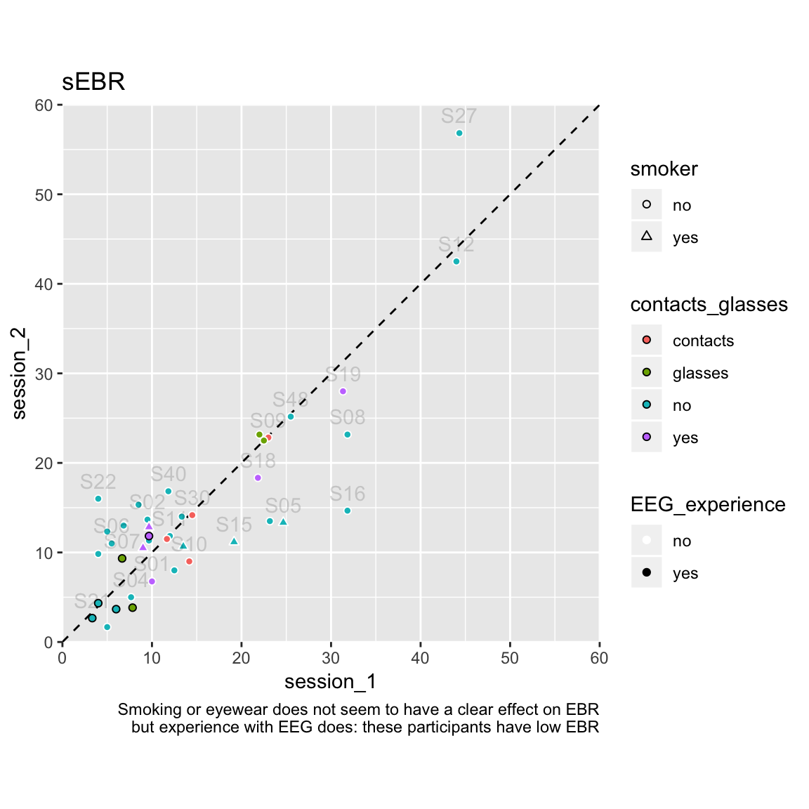
Reliability of spontaneous Eye Blink Rate
df_sEBR %>%
  left_join(df_sub_info, by = c("subject", "session", "polarity")) %>%
  group_by(EEG_experience) %>%
  summarise(n = n_distinct(subject), median_sEBR = median(sEBR)) %>%
kable(digits = 1, caption = "lower sEBR with EEG experience")| EEG_experience | n | median_sEBR |
|---|---|---|
| no | 34 | 13.3 |
| yes | 6 | 5.2 |
S27 could be classified as an outlier, because their sEBR in session 2 is the highest overall (57), and it is quite a bit higher in session 2 than in session 1 (difference of 12). This is not a data quality issue, as the blink component had little noise, and all the blinks seem to have been marked correctly.1
Statistics
Compute intra-class correlations (ICCs) for sEBR in session 1 and 2:
ICC_sEBR <- df_sEBR %>%
  select(subject, session, sEBR) %>%
  spread(session, sEBR, sep = "_") %>% # create 2 sEBR columns: session 1 and session 2
  select(-subject) %>% # drop subjects column
  ICC(lmer=FALSE) # intra-class correlation, using AOV instead of LMER (no missing data)
## Warning in if (class(x1) == as.character("try-error")) {: the condition has
## length > 1 and only the first element will be used| type | ICC | F | df1 | df2 | p | lower bound | upper bound | |
|---|---|---|---|---|---|---|---|---|
| Single_raters_absolute | ICC1 | 0.845 | 11.937 | 39 | 40 | 0 | 0.728 | 0.915 |
| Single_random_raters | ICC2 | 0.845 | 11.683 | 39 | 39 | 0 | 0.726 | 0.915 |
| Single_fixed_raters | ICC3 | 0.842 | 11.683 | 39 | 39 | 0 | 0.721 | 0.913 |
| Average_raters_absolute | ICC1k | 0.916 | 11.937 | 39 | 40 | 0 | 0.842 | 0.956 |
| Average_random_raters | ICC2k | 0.916 | 11.683 | 39 | 39 | 0 | 0.841 | 0.956 |
| Average_fixed_raters | ICC3k | 0.914 | 11.683 | 39 | 39 | 0 | 0.838 | 0.955 |
This computes all the ICCs from Shrout and Fleiss (1979).
Since this is a reliability/test-retest analysis, we want the single-rating, absolute agreement, two-way mixed effects model (or two-way random effects; same formula). This is ICC(2,1) in the conventions from Shrout and Fleiss (1979). See Koo & Li (2016) for more information.
The ICC is based on an ANOVA model, so we can also examine whether sEBR differs significantly between the sessions (and subjects, but that’s surely the case). There is no significant difference between sessions in sEBR: F(1, 39) = 0.149, p = 0.701. This is good, as at first we were worried participants would blink less in the second session, because they learned during the 1st session that blinks created artefacts in the EEG signal during task performance.
df_sEBR %>%
  left_join(df_sub_info, by = c("subject", "session", "polarity")) %>%
  group_by(session) %>%
  summarise(median_sEBR = median(sEBR)) %>%
kable(digits = 1, caption = "no difference in sEBR between sessions")| session | median_sEBR |
|---|---|
| 1 | 11.7 |
| 2 | 12.6 |
The intra-class correlation is 0.85, with a 95% confidence interval of 0.73–0.92, indicating the level of reliability is “good” (Koo & Li, 2016).
Kruis et al. (2016) report Cronbach’s alpha values over three sessions for sEBR of 0.85 (long-term meditators) and 0.79 (meditation-naive participants). This is equivalent to an average-measures two-way ICC for consistency. In our data, this ICC is 0.91, 95%CI [0.84, 0.95]
AB magnitude
Plot
Plot session 1 data against session 2:
df_ABmag %>%
  filter(block == "pre") %>%
  select(subject, session, AB_magnitude) %>%
  spread(session, AB_magnitude, sep = "_") %>%

  ggplot(aes(session_1,session_2)) +
  geom_abline(linetype = "dashed") +
  geom_point() +
  coord_equal(xlim = c(0,.75), ylim = c(0,.75), expand = FALSE) +
  labs(title = "AB magnitude", subtitle = "in baseline block")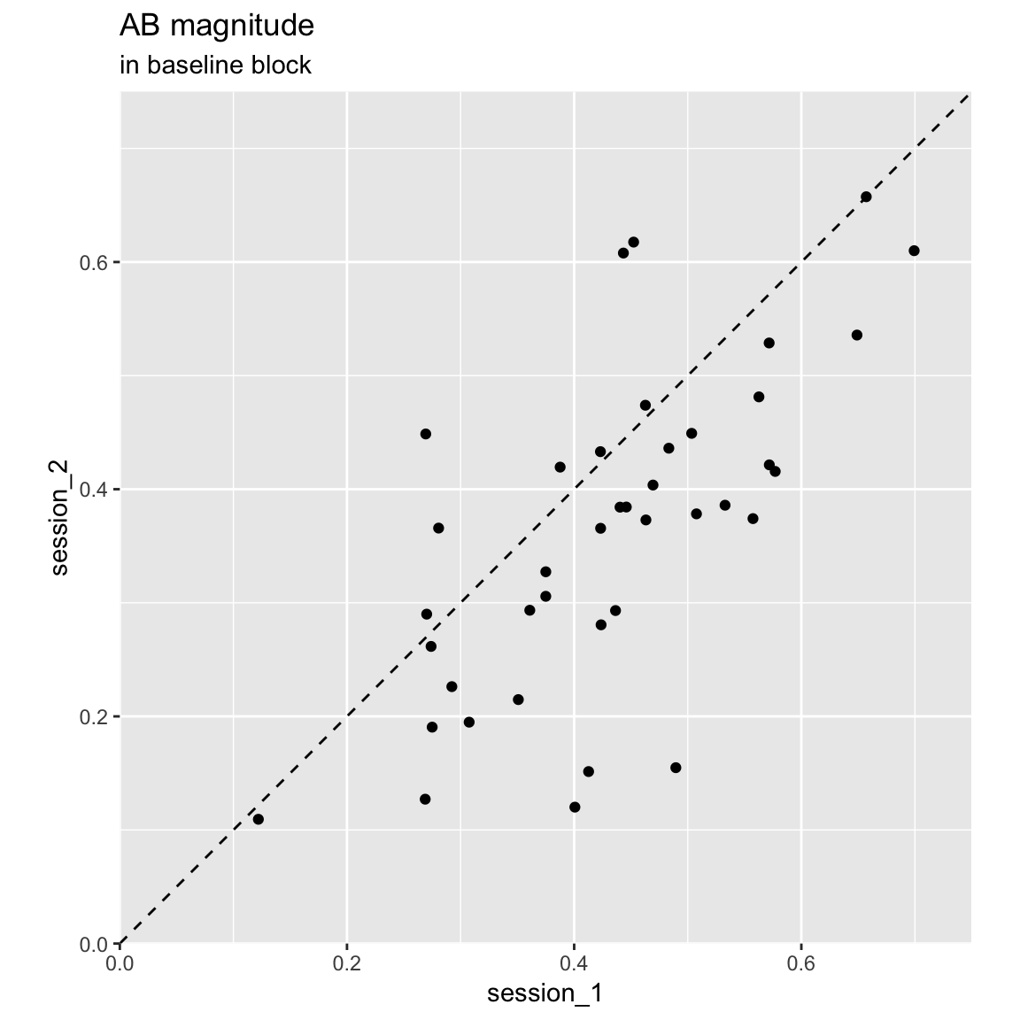
Reliability of AB magnitude
Statistics
Compute intra-class correlations for AB magnitude in session 1 and 2:
ICC_ABmag <- df_ABmag %>%
  filter(block == "pre") %>%
  select(subject, session, AB_magnitude) %>%
  spread(session, AB_magnitude, sep = "_") %>% # create 2 sEBR columns: session 1 and session 2
  select(-subject) %>% # drop subjects column
  ICC(lmer=FALSE) # intra-class correlation
## Warning in if (class(x1) == as.character("try-error")) {: the condition has
## length > 1 and only the first element will be used| type | ICC | F | df1 | df2 | p | lower bound | upper bound | |
|---|---|---|---|---|---|---|---|---|
| Single_raters_absolute | ICC1 | 0.574 | 3.694 | 39 | 40 | 0 | 0.325 | 0.749 |
| Single_random_raters | ICC2 | 0.598 | 5.128 | 39 | 39 | 0 | 0.246 | 0.790 |
| Single_fixed_raters | ICC3 | 0.674 | 5.128 | 39 | 39 | 0 | 0.461 | 0.813 |
| Average_raters_absolute | ICC1k | 0.729 | 3.694 | 39 | 40 | 0 | 0.491 | 0.856 |
| Average_random_raters | ICC2k | 0.748 | 5.128 | 39 | 39 | 0 | 0.394 | 0.882 |
| Average_fixed_raters | ICC3k | 0.805 | 5.128 | 39 | 39 | 0 | 0.631 | 0.897 |
There is a significant difference in AB magnitude between the sessions: F(1, 39) = 16.53, p = 0. This can also be seen in the scatter plot: most participants have a smaller AB magnitude in the 2nd session.
df_AB %>%
  filter(block == "pre") %>%
  mutate(session = factor(paste("session", session)),
         lag = factor(lag)) %>%
  ggplot(aes(lag,T2_given_T1)) +
  facet_wrap(~session) +
  geom_line(aes(group = subject), alpha = .25) +
  stat_summary(geom = "line", fun.y = mean, aes(group = 1)) +
  stat_summary(geom = "errorbar", fun.data = mean_se, width = 0.1)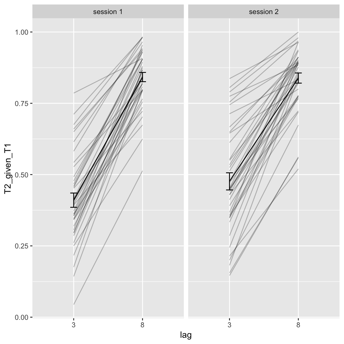
The difference in AB magnitude over sessions seems to be driven by the short lag, so the AB genuinely becomes smaller in the second session. Usually this is not the case (only T2 performance improves over time, but no interaction with lag, Dale, Dux & Arnell (2013)).
The intra-class correlation is 0.6, indicating “moderate” reliability, with a 95% confidence interval of 0.25 (poor) – 0.79 (good).
For comparison with previous studies, let’s also look at the regular Pearson correlation:
df_ABmag %>%
  filter(block == "pre") %>%
  select(subject, session, AB_magnitude) %>%
  spread(session, AB_magnitude, sep = "_") %>%
  cor.test(data = ., .$session_1, .$session_2, method = "pearson", alternative = "two.sided")
##
## Pearson's product-moment correlation
##
## data: .$session_1 and .$session_2
## t = 5.7259, df = 38, p-value = 1.354e-06
## alternative hypothesis: true correlation is not equal to 0
## 95 percent confidence interval:
## 0.4683432 0.8185404
## sample estimates:
## cor
## 0.680563This is actually in the higher range of what is typically reported: (around .4–.6, Dale, Dux & Arnell (2013)).
Correlation sEBR ~ AB magnitude
Correlations between the two measures are bounded by their reliability, but since both were good (or at least acceptable), this sets a reasonable upper bound even with our relatively limited sample size.
Linear
Colzato et al. (2009) report a negative association between sEBR and AB magnitude: participants with higher sEBR have a smaller attentional blink. However, this relationship was not replicated by Georgopoulou & Slagter (2013).
Plot
df_sEBR %>%
  left_join(df_ABmag, by = c("subject", "session", "polarity")) %>%
  left_join(df_sub_info, by = c("subject", "session", "polarity")) %>%
  filter(block == "pre") %>%
  mutate(session = paste("session", session)) %>% # add "session" to facet labels

  ggplot(aes(sEBR, AB_magnitude)) +
  facet_wrap(~session) +
  geom_point(aes(color = EEG_experience)) +
  geom_smooth(method = "lm") +
  xlab("sEBR (/min)") +
  ylab("AB magnitude in baseline block")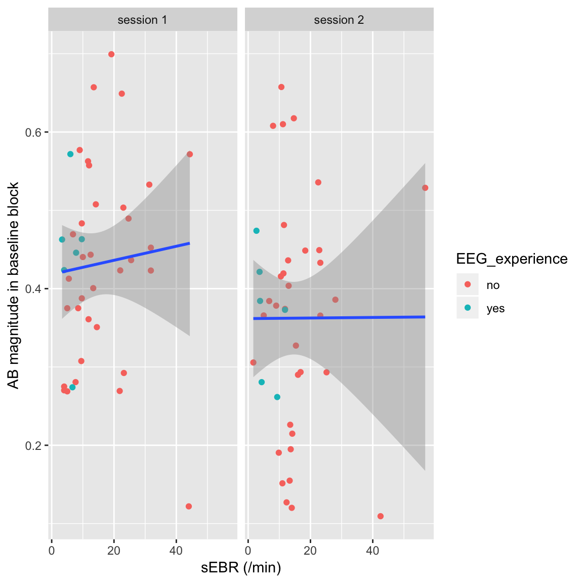
sEBR vs. AB magnitude in session 1 or 2
Pearson
lCorr <- df_sEBR %>%
  left_join(df_ABmag, by = c("subject", "session", "polarity")) %>%
  filter(block == "pre") %>% # only baseline block
  nest(-session) %>% # for each session
  mutate(stats = map(data, ~cor.test(.$sEBR, .$AB_magnitude,
                                     alternative = "two.sided",
                                     method = "pearson"))) %>% # correlate sEBR to AB magnitude
  unnest(map(stats,tidy), .drop = TRUE) # make output into data frame, drop rest

kable(lCorr, digits = 2, caption = "sEBR vs. AB magnitude correlation in either session")| session | estimate | statistic | p.value | parameter | conf.low | conf.high | method | alternative |
|---|---|---|---|---|---|---|---|---|
| 1 | 0.08 | 0.48 | 0.64 | 38 | -0.24 | 0.38 | Pearson’s product-moment correlation | two.sided |
| 2 | 0.00 | 0.02 | 0.99 | 38 | -0.31 | 0.31 | Pearson’s product-moment correlation | two.sided |
So here there’s virtually no association (even slightly positive in session 1).
Bayesian
Default
df_sEBR %>%
  left_join(df_ABmag, by = c("subject", "session", "polarity")) %>%
  filter(block == "pre") %>% # only baseline block
  nest(-session) %>% # for each session
  mutate(BF_null = 1 / map_dbl(data, ~extractBF(correlationBF(.$sEBR, .$AB_magnitude),
                     onlybf = TRUE))) %>% # correlate sEBR to AB magnitude
  select(-data) %>%
kable(digits = 2, caption = "Bayes factor (in favor of H0) sEBR vs. AB magnitude")| session | BF_null |
|---|---|
| 1 | 2.57 |
| 2 | 2.84 |
Weak evidence (bordering on moderate) for the null hypothesis of no correlations
One-sided
All prior mass folded to negative effect sizes only:
df_sEBR %>%
  left_join(df_ABmag, by = c("subject", "session", "polarity")) %>%
  filter(block == "pre") %>% # only baseline block
  nest(-session) %>% # for each session
  mutate(BF_one_sided = map(data, ~rownames_to_column(extractBF(correlationBF(.$sEBR, .$AB_magnitude, nullInterval = c(-1,0)))))) %>% # correlate sEBR to AB magnitude
  unnest(BF_one_sided, .drop = T) %>%
  mutate(BF_null = 1/ bf) %>% # transform to evidence for null
  select(-error,-time,-code,-bf) %>% # drop extra columsn in BF object
  filter(!str_detect(rowname, "!")) %>% # filter out complement to interval
  kable(digits = 2, caption = "Bayes factor (in favor of H0) with one-sided prior")
## Warning in bind_rows_(x, .id): Unequal factor levels: coercing to character## Warning in bind_rows_(x, .id): binding character and factor vector,
## coercing into character vector
## Warning in bind_rows_(x, .id): binding character and factor vector,
## coercing into character vector| session | rowname | BF_null |
|---|---|---|
| 1 | Alt., r=0.333 -1<rho<0 | 3.90 |
| 2 | Alt., r=0.333 -1<rho<0 | 2.87 |
Now the evidence for the null in the first session is a bit stronger (because there the direction of the effect is slightly positive).
Replication BF
Finally, we can specify a replication Bayes Factor [(Wagenmakers, Verhagen & Ly, 2016)]((https://doi.org/10.3758/s13428-015-0593-0) for the result in Colzato et al. (2008), who found a negative correlation: r(20) = -.530.2
lCorr %>%
  nest(-session) %>%
  mutate(bf0R = 1 / map_dbl(data, ~repBfR0(nOri = 20, rOri = -.530, nRep = .$parameter+2, rRep = .$estimate))) %>%
  select(-data) %>%
kable(digits = 2, caption = "Replication Bayes Factor (in favor of H0)")| session | bf0R |
|---|---|
| 1 | 15.80 |
| 2 | 10.43 |
There is strong evidence in favor of the null hypothesis that there is no effect, vs. the hypothesis that the effect is as in Colzato et al. (2008).
“Inverted-u-shaped”
However, the relationship between dopamine levels (indexed by sEBR) and cognitive performance is usually not characterized as linear, but inverted u-shaped (Cools & d’Esposito, 2011).
This can be examined by testing for a sign-flip in the relationship between sEBR and AB magnitude: if it is inverted u-shaped, low-sEBR values (first half of the \(\cap\)) should correlate positively with ABmagnitude, whereas high-sEBR values (second half of the \(\cap\)) should correlate negatively. The two-lines test (Simonsohn, 2019) implements this by estimating a “break point” (the apex of the \(\cap\)) from the data, and then performing two regressions.
uCorr_pre_session1 <- df_sEBR %>%
left_join(df_ABmag, by = c("subject", "session", "polarity")) %>%
filter(block == "pre", session == 1) %>%
twolines(AB_magnitude~sEBR, data = .)
title('session 1')
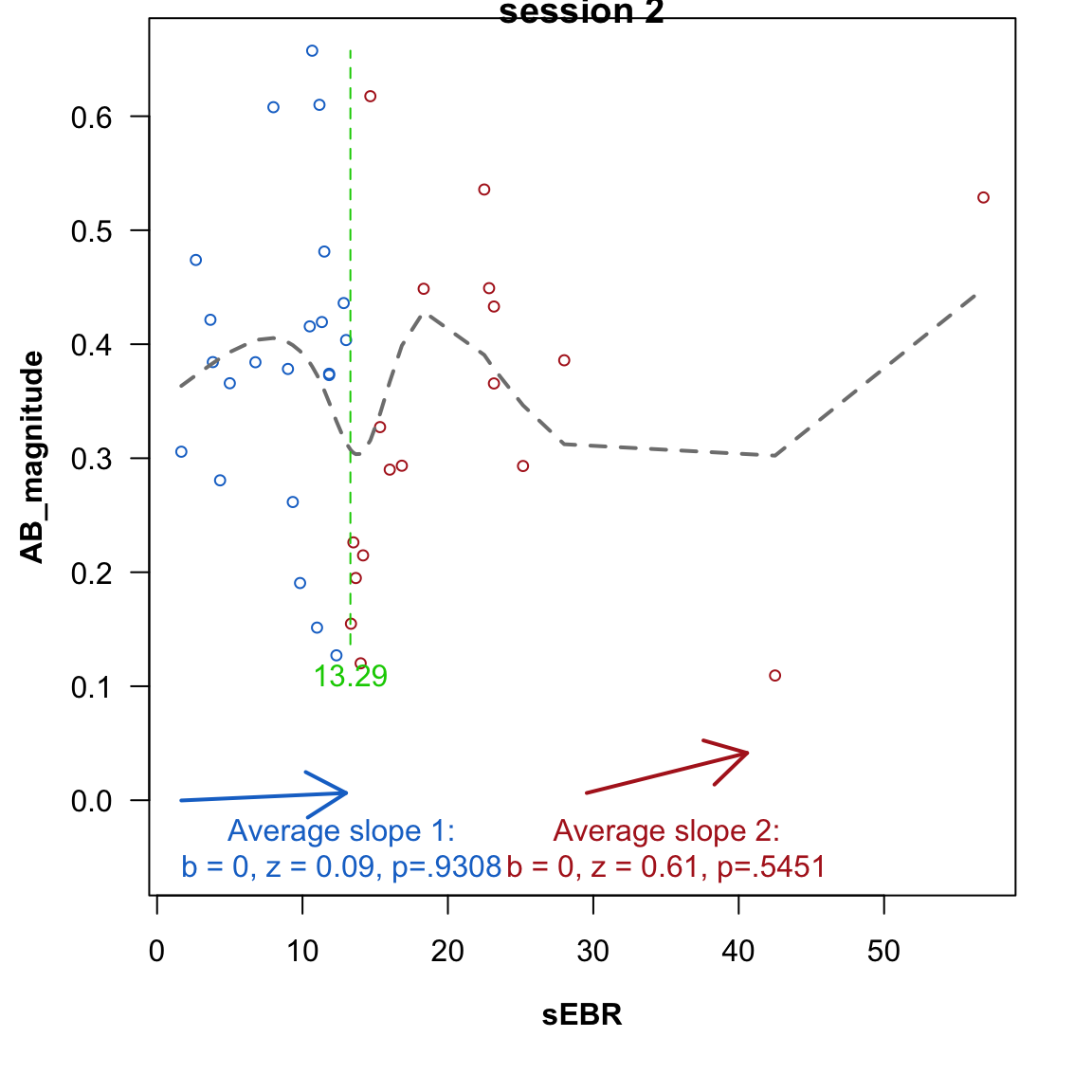
uCorr_pre_session2 <- df_sEBR %>%
left_join(df_ABmag, by = c("subject", "session", "polarity")) %>%
filter(block == "pre", session == 2) %>%
twolines(AB_magnitude~sEBR, data = .)
title('session 2')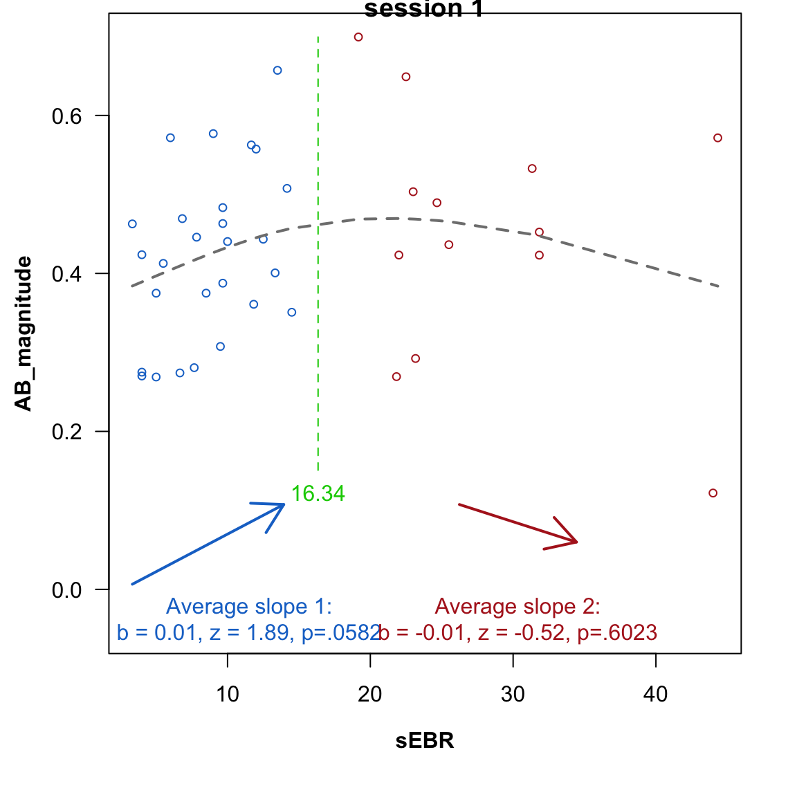
For the first session data, the overall shape is an inverted-U, but neither slope is significant (although the positive slope is trending).
The 2nd-session data looks different: there are more break-points in the cubic spline fit, and both slopes are (a tiny bit) positive. Still both-slopes are non-significant.
Correlation sEBR ~ tDCS effect on AB magnitude
Correlate AB magnitude change scores
The effects of tDCS could depend on an individual’s striatal dopamine levels. sEBR can be used as a proxy for the latter. For the former, we’ll use the “change from baseline” scores in the anodal and cathodal sessions, by subtracting baseline T2|T1 accuracy from T2|T1 accuracy during the tDCS or post blocks:
df_ABmag_change <- df_ABmag %>%
  group_by(subject,session,polarity) %>%
   summarise(`tDCS - baseline` = AB_magnitude[block == "tDCS"] - AB_magnitude[block == "pre"],
             `post - baseline` = AB_magnitude[block == "post"] - AB_magnitude[block == "pre"]) %>%
   gather(change, AB_magnitude, `tDCS - baseline`, `post - baseline`) %>%
   mutate(change = fct_relevel(change, "tDCS - baseline")) # reorder so this comes first
Plot
df_sEBR %>%
  left_join(df_ABmag_change, by = c("subject", "session", "polarity")) %>%
  ggplot(aes(sEBR, AB_magnitude)) +
  facet_grid(polarity~change) +
  geom_hline(yintercept = 0, linetype = "dashed") +
  geom_point() +
  geom_smooth(method = "lm") +
  xlab("sEBR (/min)") +
  ylab("AB magnitude change")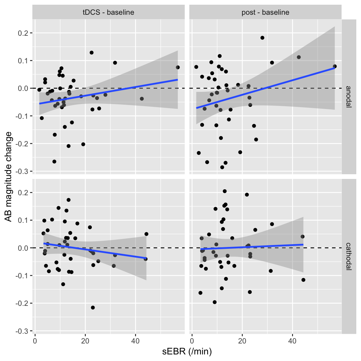
Pearson
df_sEBR %>%
  left_join(df_ABmag_change, by = c("subject", "session", "polarity")) %>%
  nest(-polarity,-change) %>% # for anodal/cathodal & during/after
  mutate(stats = map(data, ~cor.test(.$sEBR, .$AB_magnitude,
                                     alternative = "two.sided",
                                     method = "pearson"))) %>% # correlate sEBR to AB magnitude
  unnest(map(stats,tidy), .drop = TRUE) %>% # make output into data frame, drop rest
kable(digits = 2, caption = "sEBR vs. effect of tDCS correlations")| polarity | change | estimate | statistic | p.value | parameter | conf.low | conf.high | method | alternative |
|---|---|---|---|---|---|---|---|---|---|
| anodal | tDCS - baseline | 0.21 | 1.31 | 0.20 | 38 | -0.11 | 0.49 | Pearson’s product-moment correlation | two.sided |
| anodal | post - baseline | 0.24 | 1.53 | 0.13 | 38 | -0.08 | 0.51 | Pearson’s product-moment correlation | two.sided |
| cathodal | tDCS - baseline | -0.16 | -1.02 | 0.31 | 38 | -0.45 | 0.16 | Pearson’s product-moment correlation | two.sided |
| cathodal | post - baseline | 0.04 | 0.24 | 0.81 | 38 | -0.28 | 0.35 | Pearson’s product-moment correlation | two.sided |
Bayesian
df_sEBR %>%
  left_join(df_ABmag_change, by = c("subject", "session", "polarity")) %>%
  nest(-polarity,-change) %>% # for anodal/cathodal & during/after
  mutate(BF_null = 1 / map_dbl(data, ~extractBF(correlationBF(.$sEBR, .$AB_magnitude),
                     onlybf = TRUE))) %>% # correlate sEBR to AB magnitude
  select(-data) %>%
kable(digits = 2, caption = "Bayes factor (in favor of H0) sEBR vs. effect of tDCS")| polarity | change | BF_null |
|---|---|---|
| anodal | tDCS - baseline | 1.37 |
| anodal | post - baseline | 1.05 |
| cathodal | tDCS - baseline | 1.81 |
| cathodal | post - baseline | 2.77 |
Comparing the correlations in different blocks
A complementary way of looking at this is not to compute change scores, but to compute the correlation between sEBR and AB magnitude in each block.
r_ABmag_sEBR <- df_sEBR %>%
  left_join(df_ABmag, by = c("subject", "session", "polarity")) %>%
  nest(-polarity,-block) %>% # for each session
  mutate(stats = map(data, ~cor.test(.$sEBR, .$AB_magnitude,
                                     alternative = "two.sided",
                                     method = "pearson"))) %>% # correlate sEBR to AB magnitude
  unnest(map(stats,tidy), .drop = TRUE) # make output into data frame, drop rest

kable(r_ABmag_sEBR, digits = 2, caption = "sEBR vs. AB magnitude correlation per block")| polarity | block | estimate | statistic | p.value | parameter | conf.low | conf.high | method | alternative |
|---|---|---|---|---|---|---|---|---|---|
| anodal | post | 0.25 | 1.58 | 0.12 | 38 | -0.07 | 0.52 | Pearson’s product-moment correlation | two.sided |
| anodal | pre | 0.04 | 0.23 | 0.82 | 38 | -0.28 | 0.34 | Pearson’s product-moment correlation | two.sided |
| anodal | tDCS | 0.15 | 0.94 | 0.35 | 38 | -0.17 | 0.44 | Pearson’s product-moment correlation | two.sided |
| cathodal | post | 0.09 | 0.53 | 0.60 | 38 | -0.23 | 0.39 | Pearson’s product-moment correlation | two.sided |
| cathodal | pre | 0.05 | 0.29 | 0.78 | 38 | -0.27 | 0.35 | Pearson’s product-moment correlation | two.sided |
| cathodal | tDCS | -0.05 | -0.33 | 0.75 | 38 | -0.36 | 0.26 | Pearson’s product-moment correlation | two.sided |
r_ABmag_sEBR %<>% # reshape data frame for joining later
  select(polarity, block, estimate, parameter) %>% # only keep correlations, and key columns
  spread(block, estimate) %>%
  gather(block, estimate, tDCS, post) %>% # separate column for subsequent blocks
  rename(r_subsequent = estimate, r_baseline = pre) # vs. baseline
The correlations can then also be directly compared to see if they differ significantly (e.g., whether the correlation in the “pre” block in the anodal/cathodal session is significantly different than the correlation in the “tDCS” or “post blocks”).
There are lots of tests for comparing correlations implemented in the cocor package; see its accompanying paper: https://doi.org/10.1371/journal.pone.0121945.
First we need the reliability for the AB magnitude scores, i.e. the correlation between the AB magnitude scores in the different blocks:
r_ABmag <- df_ABmag %>%
  spread(block, AB_magnitude) %>% # separate column of scores for each block
  rename(baseline_AB_magnitude = pre) %>% # so we can keep "pre" as separate column
  gather(block, AB_magnitude, tDCS, post) %>% # collapse tdcs and post columns
  nest(-block,-polarity) %>% # for each tdcs/post block and anodal/cathodal
  mutate(stats = map(data, ~cor.test(.$baseline_AB_magnitude, .$AB_magnitude,
                                     alternative = "two.sided",
                                     method = "pearson"))) %>% # correlate blocks
  unnest(map(stats,tidy), .drop = TRUE)

kable(r_ABmag, digits = 2, caption = "Reliability of AB magnitude in pre vs. subsequent blocks")| polarity | block | estimate | statistic | p.value | parameter | conf.low | conf.high | method | alternative |
|---|---|---|---|---|---|---|---|---|---|
| anodal | tDCS | 0.84 | 9.40 | 0 | 38 | 0.71 | 0.91 | Pearson’s product-moment correlation | two.sided |
| cathodal | tDCS | 0.82 | 8.78 | 0 | 38 | 0.68 | 0.90 | Pearson’s product-moment correlation | two.sided |
| anodal | post | 0.63 | 4.99 | 0 | 38 | 0.40 | 0.79 | Pearson’s product-moment correlation | two.sided |
| cathodal | post | 0.71 | 6.15 | 0 | 38 | 0.51 | 0.83 | Pearson’s product-moment correlation | two.sided |
r_ABmag %<>% # reshape data frame for joining
  select(polarity,block,estimate) %>%
  rename(r_reliability = estimate)
Now make a single table out of the 1) sEBR ~ AB magnitude correlations in each session/block 2) the pre-tDCS/pre-post reliabilities, where:
- The
r_baselinecolumn has the correlation between AB magnitude and sEBR in the baseline block, for eachpolarity - The
r_subsequentcolumn houses the same correlation for the tDCS and post blocks (indicated by theblockcolumn) - The
r_reliabilitycolumn houses the correlation between AB magnitude in the pre block and one of the subsequent blocks (tDCS or post, indicated by theblockcolumn)
## Joining, by = c("polarity", "block")| polarity | parameter | r_baseline | block | r_subsequent | r_reliability |
|---|---|---|---|---|---|
| anodal | 38 | 0.04 | tDCS | 0.15 | 0.84 |
| cathodal | 38 | 0.05 | tDCS | -0.05 | 0.82 |
| anodal | 38 | 0.04 | post | 0.25 | 0.63 |
| cathodal | 38 | 0.05 | post | 0.09 | 0.71 |
Now we have all the information to perform a significance test of the 4 correlation pairs:
corr_co_tbl <- r_corr_co %>%
  nest(-polarity, -block) %>% # for each polarity and block
  mutate(stats = map(data, ~cocor.dep.groups.overlap(.$r_baseline, .$r_subsequent, .$r_reliability,
                                     n = .$parameter + 2, return.htest = TRUE))) %>% # compare correlations
  # This yields a nested list of 10 different statistical test, for each 4 comparsions
  unnest(stats, .drop = TRUE) %>% # peel off first layer
  mutate(method = as.character(map(stats, "method"))) %>% # add column identifying lists with this method
  filter(method == "Pearson and Filon's z (1898)") %>% # keep only them
  select(-method) %>%
  unnest(map(stats,tidy), .drop = TRUE) # unnest lists into table
To fully characterize the correlation between sEBR and AB magnitude change scores, in addition to the three columns in the data frame, we’d also have to look at the difference in varability in AB magnitude scores between the blocks. See also Gardner & Neufeld (1987) and Griffin, Murray, & Gonzalez (1999).
df_ABmag %>%
  group_by(polarity,block) %>%
  summarise(SD = sd(AB_magnitude)) %>%
  spread(block,SD) %>%
  mutate(M_tDCS = tDCS/pre, M_post = post/pre) %>%
kable(caption = "Standard deviations for AB magnitude per block, as well as the ratio between the pre- and subsequent blocks (M)")| polarity | post | pre | tDCS | M_tDCS | M_post |
|---|---|---|---|---|---|
| anodal | 0.1365154 | 0.1395991 | 0.1479759 | 1.0600060 | 0.9779101 |
| cathodal | 0.1195923 | 0.1362417 | 0.1281921 | 0.9409165 | 0.8777948 |